Plot a global map from finite volume (FV) grid field (Plot_2D application)
# By line: DSJ 10-MAR-2021
# Script aims to:
# - Plot a world map with coastlines, lon/lat lines, and colorbar
# - Change colormap of the plot
# - Add unit to the plot
# - Add title to the plot
# - Manually set maximum and minimum values of the plot
At the start of a Jupyter notebook you need to import all modules that you will use
# Make sure you have downloaded "Plot_2D.py" script from Github
from Plot_2D import Plot_2D
import xarray as xr # To read NetCDF file
import matplotlib.cm as cm # To change colormap used in plots
Read the sample file
# Make sure you have downloaded "sample.nc" file from Github
ds = xr.open_dataset( 'sample.nc' )
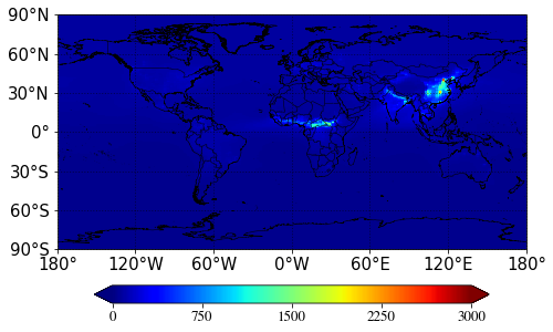
Call Plot_2D script to plot surface CO
Plot_2D( ds['CO'][0,-1,:,:]*1e9 ) # multiply by 1e9 to make it to ppbv
<Plot_2D.Plot_2D at 0x28746bb9b88>
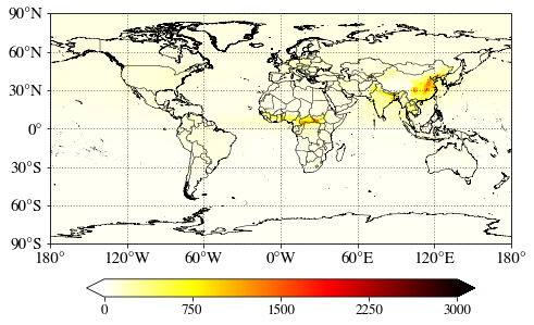
You can specify colormap. For more information, you can check colormaps from here: https://matplotlib.org/stable/tutorials/colors/colormaps.html
Plot_2D( ds['CO'][0,-1,:,:]*1e9, cmap=cm.hot_r )
<Plot_2D.Plot_2D at 0x2874c3c5588>
Let’s add an unit to the plot by using unit keyword
Plot_2D( ds['CO'][0,-1,:,:]*1e9, cmap=cm.hot_r, unit='ppbv' )
<Plot_2D.Plot_2D at 0x2874c655a08>
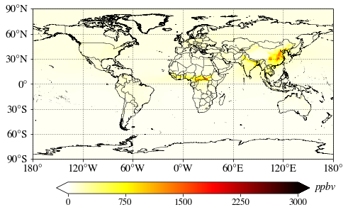
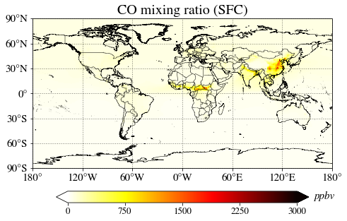
You can also add a title to the plot
Plot_2D( ds['CO'][0,-1,:,:]*1e9, cmap=cm.hot_r, unit='ppbv', title='CO mixing ratio (SFC)' )
<Plot_2D.Plot_2D at 0x2874c71ac48>
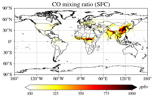
Set maximum and minimum values manually with cmin and cmax keywords
Plot_2D( ds['CO'][0,-1,:,:]*1e9, cmap=cm.hot_r, unit='ppbv', title='CO mixing ratio (SFC)',
         cmax=1000, cmin=100 )
<Plot_2D.Plot_2D at 0x2874c980788>