The VAPOR user interface enables scientists to visualize both large- and small-scale features of time-varying data sets. Its interactive 3D visualization environment runs on most UNIX, Mac OS X, and Windows systems that are equipped with modern 3D graphics cards. We provide binary installers that work on all supported platforms and we strongly recommend using a binary distribution for your installation.
The documentation and demonstration below outline and illustrate some basic steps to help you get started using VAPOR. It is intended for general use but also contains some information specific to NCAR/UCAR systems. We also provide example data sets, usage guides, and reference material on these Documentation and Training pages.
Installing VAPOR
- Read the Release Notes for the current version.
- Download the appropriate install package for your platform. (Login required.)
- Follow the installation instructions for your platform.
Preparing data
Prepare your data set as described in VAPOR Data Preparation. This is optional with some model outputs such as WRF-ARW, MOM4, CAM, and GRIMs. Output from these models can be visualized directly, with no data preparation. Some example data sets are provided here.
You will want to have your data in place in a directory of your own before you start the VAPOR interface.
Getting help
Help is available a number of ways:
- See the Documentation and Support menus above.
- Tool tips, which appear when you hold your mouse over a button or input field.
- Context-sensitive help within VAPOR. Select Explain This from the Help menu (Figure 1), then click the feature you would like to have explained.
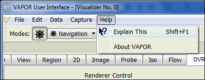
Figure 1 - Click to see an image of the VAPOR screen.
Starting VAPOR
Launch the VAPOR GUI by following the procedures for your own platform. (Starting it with vglrun, as in this example, is specific for NCAR/UCAR users running on the Geyser or Caldera clusters.)
vglrun vaporgui
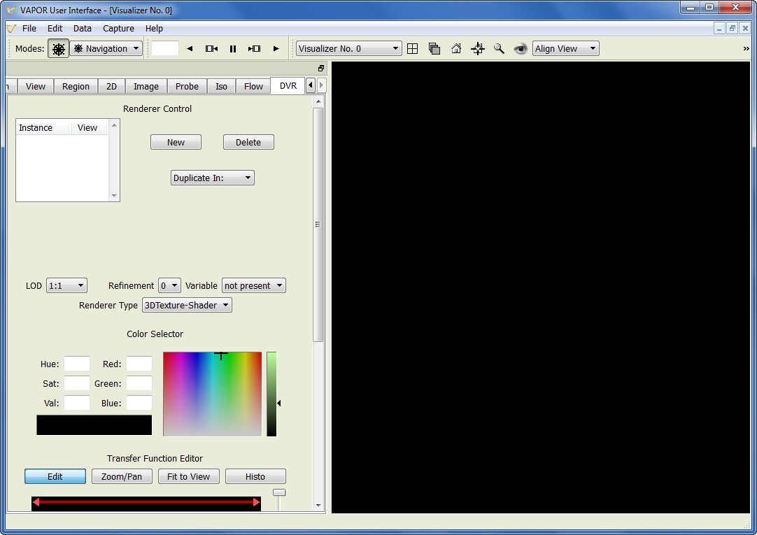
Figure 2 - Click to enlarge.
With the VAPOR interface open (Figure 2), you can load your data set and proceed.
The following visualization example demonstrates some basic VAPOR functions.
Visualization example using WRF-ARW
This documentation will be most helpful if you refer to it after starting VAPOR as described above, then work through the example to create a basic visualization.
Steps
- Load your data set
- Stretch the scene
- Display an image
- Define a variable
- Edit the transfer function
- Capture an animation
Loading a data set
This example assumes that you have copied these sample WRF-ARW data files from the ftp site to a directory on your own system.
Substitute your own directory name and data set as appropriate.
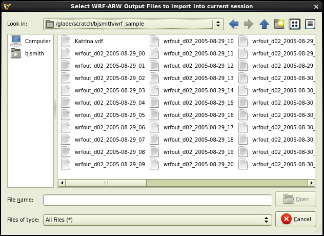
Figure 3 - Click to enlarge.
Procedure:
- From the Data menu at the top of the VAPOR window, click Import data into current session, then WRF-ARW.
- Use the Look in dropdown to locate your file. (Figure 3)
- Select all of the files you will be visualizing and click Open.
- A flat rectangle will appear on the screen to indicate the bounds of the current region. Stretch the scene.
Once the scene is established, you can manipulate it as follows.
- Rotate the scene by clicking and dragging with your left mouse button.
- Zoom in and out by dragging your right mouse button up and down.
- Move it horizontally or vertically by dragging with your middle mouse button.
Stretching a scene
You may need to adjust the “scene stretch” to visualize 3D data effectively. For example, if the box is 1,000 km long and 1,000 km wide but only 20 km high, the scene will be quite flat in the Z dimension.
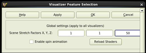
Figure 4 - Click to see the whole panel.
Procedure:
- From the Edit menu at the top of your VAPOR window, click Edit Visualizer Features. The editor will open in a new window. (Figure 4)
- Enter 50 for scene stretch factor Z.
- Click OK at the top of the panel.
The box in the scene will be taller, as will the portion of the terrain in the scene.
Displaying images
Display a background image to help you see the geographic area associated with the data you are visualizing.
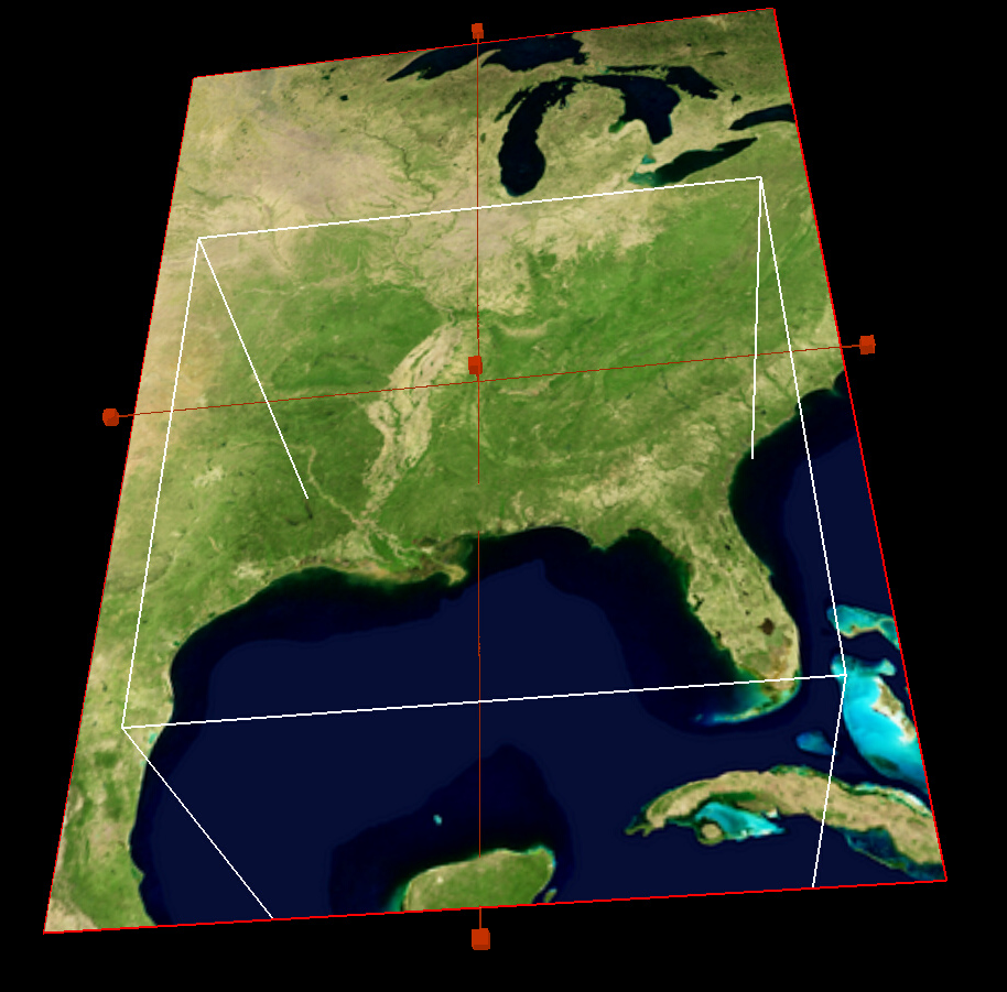
Figure 5 - Click to enlarge.
Procedure:
- Select the Image tab.
- Click Select Installed Image, then choose the background image you want to use – BigBlueMarble.tiff, for example. (If you retrieved a different terrain image, choose Select Image File instead and locate that image.)
- Check Apply to terrain.
- Check the View box next to Instance: 1. A small portion of the image will be visible.
- Select Image from the Modes dropdown menu.
- Right click the red image handles (Figure 5) and drag them to expand the portion of the image that will be visible.
- Uncheck and then recheck the View box next to Instance: 1.
Defining and selecting a variable to visualize
You can either select a variable to visualize from the Variable dropdown list or define a new variable.
For this demonstration, define a variable and add it to the dropdown list as follows.
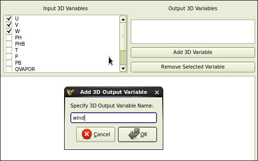
Figure 6 - Click to see the whole panel.
Procedure:
- From the Edit menu, click Edit Python program defining a new variable.
- Click the checkboxes for variables U, V, and W in the Input 3D Variables box. (Figure 6)
- Click Add 3D variable.
- Name the new variable "wind" and click OK.
- In the input field, type: wind = sqrt(U*U+V*V+W*W)
- Click Test to confirm that you did that correctly. (If the result is not "Successful Test," double-check the previous steps.)
- Click Apply after conducting a successful test.
See Using Python with VAPOR for related information.
After defining the new variable, take these additional steps:
- Click the DVR tab.
- Select the wind variable from the Variable dropdown list.
- Check the View box next to Instance: 1.
Editing the transfer function
The Transfer Function Editor controls colors and opacity in the volume rendering of your data.
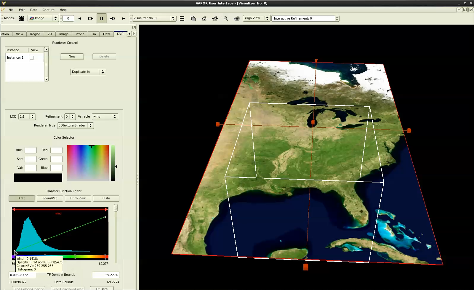
Figure 7 - Click to enlarge.
Procedure:
- Select the DVR tab. (Figure 7)
- Choose your new wind variable from the Variable menu.
- Click Fit Data, then Fit to View, then Histo.
- Click Load Installed TF button (near the bottom of the control panel) and select pre-installed transfer function reversed.vtf. This reverses the color map so larger values (greater wind speeds, for example) are red and smaller values are violet.
- Select the variable interval to be mapped to color and opacity. For example, drag the left end of the arrow at the top of the Transfer Function Editor (Figure 8) to the right about one-third (1/3) of the way to exclude low wind values.
- Reduce the opacity at the two middle control points by dragging them downward to help you see the higher wind values inside the hurricane.
- Move the opacity slider down until you can see the most useful representation of your data.
- Click Fit to View and Histo.
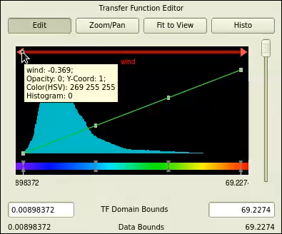
Figure 8 - Click for another view of the Transfer Function Editor.
Capturing an animation sequence
Before animating and capturing the visualization, you may want to further define or restrict the region you’re observing by rotating the scene, zooming in or out, or changing the size of the region box.
Then, use the VAPOR animation toolbar or “player” to animate and capture a sequence of the visualization. (Figure 9)

Figure 9 - Click to enlarge.
Procedure:
To capture the animation sequence, proceed as follows.
- From the Mode menu near the top of your VAPOR window, select Navigation.
- Set the current time step to 1.
- Zoom in to get a close look at the hurricane
- From the Capture menu at the top of your VAPOR window, select Begin image capture sequence.
- Choose a name for the jpeg files to be captured — "KatrinaEye.jpg,” for example.
- Click the Play Forward button on the animation toolbar, and watch the animation proceed to its completion.
- From the Capture menu, select End image capture sequence.
VAPOR saves a series of jpeg files to disk. You can convert them into a movie file using any of various utilities such as QuickTime Pro and FFmpeg.