EOF analysis - x4c: Xarray for CESM

Empirical orthogonal functions are one of the things that come up constantly and are easy to get wrong by hand.

import os
import numpy as np
import xarray as xr
import matplotlib.pyplot as plt
import nc_time_axis  # registers the cftime axis converter for matplotlib
import x4c

x4c.set_style('journal')

# after set_style: it resets rcParams from matplotlibrc defaults, which includes the
# backend, so assert the inline backend last or figures are never captured
%matplotlib inline

# The tutorial runs against a reduced copy of a real CESM case. It is published as a
# GitHub Release asset rather than committed, so the first call downloads it into
# ~/.cache/x4c (override with $X4C_CACHE_DIR) and later calls reuse it. Set
# $X4C_SAMPLE_DIR to point at a copy you already have.
case_dir = x4c.fetch_sample_data(case='cesm1', verbose=False)
casename = os.path.basename(case_dir)
print('x4c', x4c.__version__)

x4c 2026.6.11

case = x4c.Timeseries(case_dir, grid_dict={'atm': 'ne16np4', 'ocn': 'g16'},
                      cesm_ver=1)
case.load('TS', timespan=(1, 10), verbose=False)

# EOFs need a regular grid, so regrid off the spectral-element grid first
ts = case.ds['TS'].x.regrid(2, 2).x.da
print(dict(ts.sizes))

>>> case.root_dir: /glade/u/home/fengzhu/.cache/x4c/sample_data/cesm1_sample_data/b.e13.B1850C5.ne16_g16.icesm131_d18O_fixer.Miocene.3xCO2.005
>>> case.path_pattern: comp/proc/tseries/*/casename.hstr.vn.timespan.nc
>>> case.grid_dict: {'atm': 'ne16np4', 'ocn': 'g16', 'lnd': 'ne16np4', 'rof': 'ne16np4', 'ice': 'g16'}
>>> case.casename: b.e13.B1850C5.ne16_g16.icesm131_d18O_fixer.Miocene.3xCO2.005
>>> case.paths["atm"]["cam.h0"] created
>>> case.paths["ocn"]["pop.h"] created
>>> case.paths["lnd"]["clm2.h0"] created
>>> case.paths["ice"]["cice.h"] created
>>> case.vns["atm"]["cam.h0"] created
>>> case.vns["ocn"]["pop.h"] created
>>> case.vns["lnd"]["clm2.h0"] created
>>> case.vns["ice"]["cice.h"] created

{'time': 120, 'lat': 90, 'lon': 180}

Grid predicates¶

.x.plot() uses these to decide what kind of plot to draw; they are also handy in your own code when a function has to accept either a native or a regridded field.

native = case.ds['TS'].x.da
print('native  : is_cam_se', native.x.is_cam_se(), '| is_latlon', native.x.is_latlon(),
      '| is_map', native.x.is_map())
print('regridded: is_cam_se', ts.x.is_cam_se(), '| is_latlon', ts.x.is_latlon(),
      '| is_map', ts.x.is_map())
print('a timeseries is not a map:', ts.x.gm.x.is_map())

native  : is_cam_se True | is_latlon False | is_map True
regridded: is_cam_se False | is_latlon True | is_map True
a timeseries is not a map: False

EOF analysis¶

.x.eof(n) returns (pcs, eofs, variance_fractions). The field is weighted by sqrt(cos(lat)) first so that the modes are area-fair rather than dominated by the poles — pass weight=False to skip that.

anom = ts.x.anom                     # remove the monthly climatology first
pcs, eofs, var = anom.x.eof(n=3)

print('PCs  :', dict(pcs.sizes))
print('EOFs :', dict(eofs.sizes))
print('variance explained:', np.round(var.values * 100, 1), '%')

PCs  : {'time': 120, 'mode': 3}
EOFs : {'mode': 3, 'lat': 90, 'lon': 180}
variance explained: [17.3 10.2  7.6] %

ssh_path = os.path.join(case_dir, 'ocn', 'proc', 'tseries', 'month_1',
                        f'{casename}.pop.h.SSH.000101-000512.nc')
ssv = x4c.open_dataset(ssh_path, comp='ocn', grid='g16', vn='SSH',
                       shift_time=True).x.regrid().x.da.mean('time')

ax_loc = {'a': (0, 0), 'b': (0, 1)}
fig, axd = x4c.subplots(1, 2, ax_loc=ax_loc,
                        projs={k: 'Robinson' for k in ax_loc},
                        projs_kws={k: {'central_longitude': 180} for k in ax_loc},
                        figsize=(13, 3.4), wspace=0.15,
                        annotation=True)

for i, k in enumerate(['a', 'b']):
    m = eofs.isel(mode=i)
    m.attrs['long_name'] = f'EOF{i + 1} ({var.values[i] * 100:.1f}% of variance)'
    m.x.plot(ax=axd[k], ssv=ssv, cmap='RdBu_r', levels=np.linspace(-2, 2, 17),
             title=m.attrs['long_name'])
x4c.showfig(fig)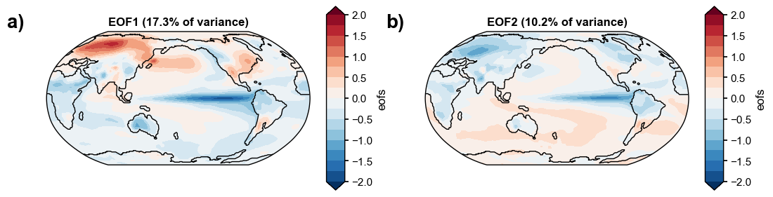

annotation=True on x4c.subplots adds the a) b) panel labels; x4c.add_annotation does the same to axes you built yourself.

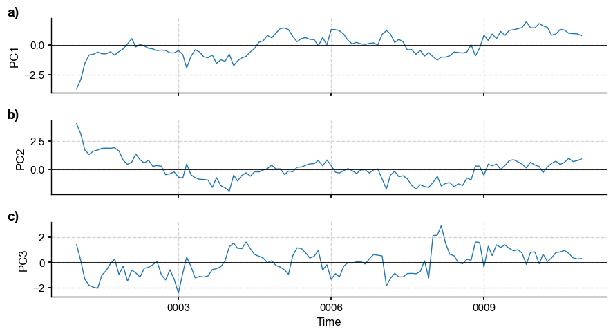
fig, axes = plt.subplots(3, 1, figsize=(9, 5), sharex=True)
for i, axi in enumerate(axes):
    axi.plot(pcs.time, pcs.isel(mode=i), lw=1)
    axi.axhline(0, color='k', lw=0.6)
    axi.set_ylabel(f'PC{i + 1}')
axes[-1].set_xlabel('Time')
x4c.add_annotation(list(axes), style=')', loc_x=-0.08, fs=14)
fig.tight_layout()
x4c.showfig(fig)