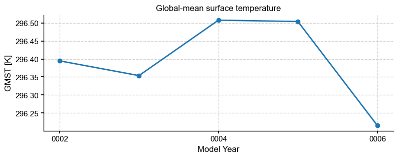
1-D data takes the line branch.
import os
import numpy as np
import xarray as xr
import matplotlib.pyplot as plt
import nc_time_axis  # registers the cftime axis converter for matplotlib
import x4c

x4c.set_style('journal')

# after set_style: it resets rcParams from matplotlibrc defaults, which includes the
# backend, so assert the inline backend last or figures are never captured
%matplotlib inline

# The tutorial runs against a reduced copy of a real CESM case. It is published as a
# GitHub Release asset rather than committed, so the first call downloads it into
# ~/.cache/x4c (override with $X4C_CACHE_DIR) and later calls reuse it. Set
# $X4C_SAMPLE_DIR to point at a copy you already have.
case_dir = x4c.fetch_sample_data(case='cesm1', verbose=False)
casename = os.path.basename(case_dir)
print('x4c', x4c.__version__)
x4c 2026.6.11
ts_path = os.path.join(
    case_dir, 'atm', 'proc', 'tseries', 'month_1',
    f'{casename}.cam.h0.TS.000101-000512.nc',
)
ds = x4c.open_dataset(ts_path, comp='atm', grid='ne16np4', vn='TS', shift_time=True)
gmst = ds.x.da.x.annualize().x.gm
fig, ax = gmst.x.plot(figsize=(9, 3), marker='o')
ax.set(title='Global-mean surface temperature', ylabel='GMST [K]')
x4c.showfig(fig)