Spatial means and climate indices - x4c: Xarray for CESM

All of the spatial reductions are area-weighted using the grid metadata that x4c attached when the file was opened.

import os
import numpy as np
import xarray as xr
import matplotlib.pyplot as plt
import nc_time_axis  # registers the cftime axis converter for matplotlib
import x4c

x4c.set_style('journal')

# after set_style: it resets rcParams from matplotlibrc defaults, which includes the
# backend, so assert the inline backend last or figures are never captured
%matplotlib inline

# The tutorial runs against a reduced copy of a real CESM case. It is published as a
# GitHub Release asset rather than committed, so the first call downloads it into
# ~/.cache/x4c (override with $X4C_CACHE_DIR) and later calls reuse it. Set
# $X4C_SAMPLE_DIR to point at a copy you already have.
case_dir = x4c.fetch_sample_data(case='cesm1', verbose=False)
casename = os.path.basename(case_dir)
print('x4c', x4c.__version__)

x4c 2026.6.11

fpath = os.path.join(
    case_dir, 'atm', 'proc', 'tseries', 'month_1',
    f'{casename}.cam.h0.TS.000101-000512.nc',
)
ds = x4c.open_dataset(fpath, comp='atm', grid='ne16np4', vn='TS', shift_time=True)
da = ds.x.da.x.annualize()
da

Global and hemispheric¶

gm/nhm/shm are means; gs/nhs/shs are the corresponding area-weighted sums. All are properties, not methods.

print(f'global mean : {float(da.x.gm[0]):8.3f} K')
print(f'NH mean     : {float(da.x.nhm[0]):8.3f} K')
print(f'SH mean     : {float(da.x.shm[0]):8.3f} K')
print()
print(f'global sum  : {float(da.x.gs[0]):.4e} K m^2')

global mean :  296.395 K
NH mean     :  295.597 K
SH mean     :  297.059 K

global sum  : 3.7246e+03 K m^2

The weight has to span dimensions the data actually has. If it does not — which can happen if you build a DataArray by hand and attach a mismatched weight — the reduction refuses rather than silently broadcasting into a much larger array.

bad = da.copy()
bad.attrs['gw'] = xr.DataArray(np.ones(10), dims='not_a_real_dim')
try:
    bad.x.gm
except ValueError as e:
    print('ValueError:', str(e)[:150], '...')

ValueError: The area weight `gw` spans dims ('not_a_real_dim',), which are not all present in the data dims ('time', 'ncol') (missing: ['not_a_real_dim']). The we ...

Zonal mean¶

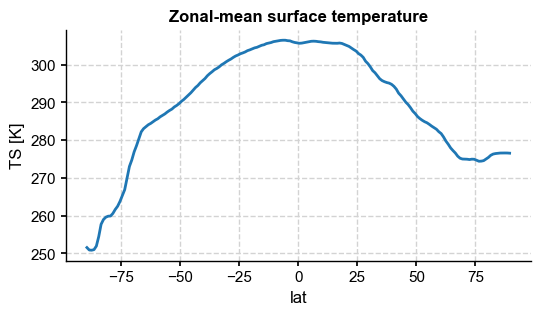
.x.zm averages over longitude. On an unstructured grid there is no longitude axis to average over, so zm regrids to a regular grid first.

zm = da.x.zm
print(zm.dims, zm.shape)

fig, ax = zm.mean('time').x.plot(title='Zonal-mean surface temperature')
x4c.showfig(fig)

('time', 'lat') (5, 180)

Regional means¶

geo_mean takes an explicit latlon_range as (lat_min, lat_max, lon_min, lon_max), with longitudes in 0-360.

tropics = da.x.geo_mean(latlon_range=(-30, 30, 0, 360))
southern = da.x.geo_mean(latlon_range=(-90, -60, 0, 360))

print(f'tropical mean (30S-30N) : {float(tropics[0]):.3f} K')
print(f'polar mean (90S-60S)    : {float(southern[0]):.3f} K')

tropical mean (30S-30N) : 304.868 K
polar mean (90S-60S)    : 275.178 K

Named climate indices¶

Common index boxes are built in, so you do not have to remember the coordinates. Available: nino3.4, nino1+2, nino3, nino4, wpi, tpi, dmi, iobw.

monthly = ds.x.da  # indices are usually computed on monthly data
for ind in ['nino3.4', 'nino3', 'nino4', 'wpi']:
    v = monthly.x.geo_mean(ind=ind)
    print(f'{ind:9s} mean over the record: {float(v.mean()):.3f} K')

nino3.4   mean over the record: 305.432 K
nino3     mean over the record: 304.802 K
nino4     mean over the record: 306.208 K
wpi       mean over the record: 307.178 K

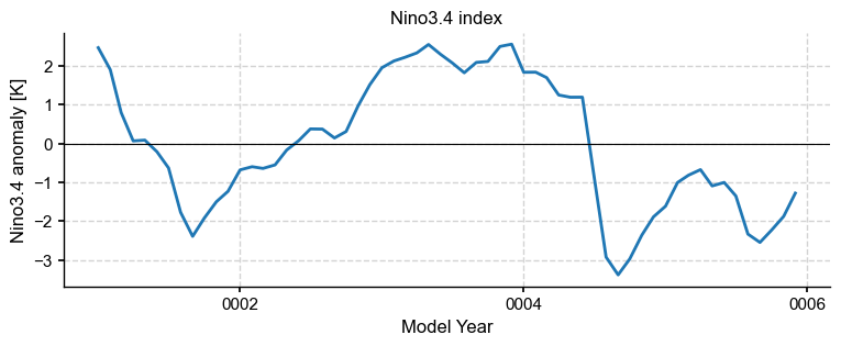
nino34 = monthly.x.geo_mean(ind='nino3.4')
nino34_anom = nino34 - nino34.mean('time')

fig, ax = nino34_anom.x.plot(figsize=(9, 3))
ax.axhline(0, color='k', lw=0.8)
ax.set(ylabel='Nino3.4 anomaly [K]', title='Nino3.4 index')
x4c.showfig(fig)