Overview - x4c: Xarray for CESM

x4c attaches a .x accessor to xarray.Dataset and xarray.DataArray that knows about CESM conventions: which variable holds the grid-cell areas, where latitude and longitude live on an unstructured grid, and how the vertical coordinate is spaced.

Everything in this tutorial runs against a reduced sample of a real case that ships with the docs — a Miocene 3xCO2 iCESM1.3 run on the ne16np4 atmosphere and g16 ocean grids. See README.md in the case directory for what was trimmed.

import os
import numpy as np
import xarray as xr
import matplotlib.pyplot as plt
import nc_time_axis  # registers the cftime axis converter for matplotlib
import x4c

x4c.set_style('journal')

# after set_style: it resets rcParams from matplotlibrc defaults, which includes the
# backend, so assert the inline backend last or figures are never captured
%matplotlib inline

# The tutorial runs against a reduced copy of a real CESM case. It is published as a
# GitHub Release asset rather than committed, so the first call downloads it into
# ~/.cache/x4c (override with $X4C_CACHE_DIR) and later calls reuse it. Set
# $X4C_SAMPLE_DIR to point at a copy you already have.
case_dir = x4c.fetch_sample_data(case='cesm1', verbose=False)
casename = os.path.basename(case_dir)
print('x4c', x4c.__version__)

x4c 2026.6.11

Opening a file¶

x4c.open_dataset is xarray.open_dataset plus two things: time is always decoded with cftime (so long paleo calendars and noleap work), and the CESM grid metadata is attached to ds.attrs.

fpath = os.path.join(
    case_dir, 'atm', 'proc', 'tseries', 'month_1',
    f'{casename}.cam.h0.TS.000101-000512.nc',
)

ds = x4c.open_dataset(fpath, comp='atm', grid='ne16np4', vn='TS', shift_time=True)
ds

shift_time=True is the CESM1 convention fix: CESM writes a monthly mean with the timestamp of the end of the averaging period, so January’s mean is stamped 1 February. Shifting it back makes .groupby('time.month') and seasonal selection mean what you expect.

What the accessor added¶

The grid metadata lands in .attrs. gw is the area weight, and for an ne16np4 spectral-element grid it comes from the area variable rather than being derived from a latitude axis — there is no latitude axis on an unstructured grid.

for k in ['comp', 'grid', 'vn']:
    print(f'{k:6s} = {ds.attrs[k]}')

print()
print('gw  :', ds.attrs['gw'].name, dict(ds.attrs['gw'].sizes))
print('lat :', ds.attrs['lat'].name, dict(ds.attrs['lat'].sizes))
print('lon :', ds.attrs['lon'].name, dict(ds.attrs['lon'].sizes))

comp   = atm
grid   = ne16np4
vn     = TS

gw  : area {'ncol': 13826}
lat : lat {'ncol': 13826}
lon : lon {'ncol': 13826}

From Dataset to DataArray¶

ds.x.da returns the variable named in ds.attrs['vn'], carrying the grid metadata with it. That is what makes the reductions below work on a bare DataArray.

da = ds.x.da
print(da.name, da.dims, da.shape)
print('carries gw?', 'gw' in da.attrs)
da

TS ('time', 'ncol') (60, 13826)
carries gw? True

Area-weighted means¶

.x.gm is the global area-weighted mean. On the native SE grid the weights are the element areas, so no regridding is needed to get a correct global mean.

gmst = da.x.gm
print('global mean surface temperature, first 5 months (K):')
print(np.round(gmst.values[:5], 3))

print()
print('NH mean:', float(da.x.nhm[0]).__round__(3))
print('SH mean:', float(da.x.shm[0]).__round__(3))

global mean surface temperature, first 5 months (K):
[294.839 295.472 296.058 296.618 297.118]

NH mean: 289.007

SH mean: 300.502

A quick sanity check that the weighting is doing real work: the unweighted mean over ncol is different, because SE elements are not equal-area.

weighted = float(da.isel(time=0).x.gm)
naive = float(da.isel(time=0).mean('ncol'))
print(f'area-weighted : {weighted:.4f} K')
print(f'unweighted    : {naive:.4f} K')
print(f'difference    : {weighted - naive:+.4f} K')

area-weighted : 294.8395 K
unweighted    : 294.8816 K
difference    : -0.0421 K

A first map¶

.x.plot() dispatches on the dimensions it finds. With ncol present it draws the unstructured grid directly with tricontourf, no regridding involved.

fig, ax = da.isel(time=0).x.plot(title='Surface temperature, month 1')
x4c.showfig(fig)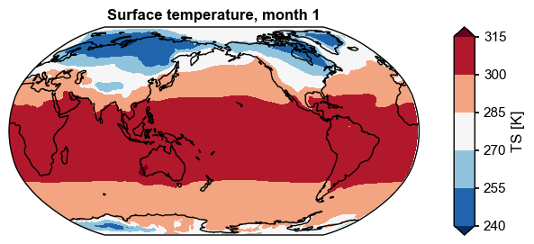

Those are modern coastlines drawn by Cartopy, which are wrong for a Miocene run. Visualization shows how to draw the model’s own coastlines instead.