Porting the diagnostics to HadCM3

x4c.Timeseries reads CESM output by default, but the same class can read other models’ output when given a model spec: a translation table from CESM-style variable names to the model’s own (vn_dict), a filename template that explains the folder structure (path_pattern), and a mapping of dimension names (dim_map). Once loaded, variables carry the same metadata as CESM output, so .x.gm, .x.plot, case.calc and the derived variables in x4c.diags work unchanged.

This notebook runs on the iHadCM3 climatologies under /glade/campaign/univ/umcp0052/data/iHadCM3/Data, using the built-in hadcm3 spec.

import numpy as np
import xarray as xr
import matplotlib.pyplot as plt
import cartopy.crs as ccrs
import x4c

x4c.set_style('journal')

# after set_style: it resets rcParams from matplotlibrc defaults, which includes the
# backend, so assert the inline backend last or figures are never captured
%matplotlib inline

root = '/glade/campaign/univ/umcp0052/data/iHadCM3/Data'

The folder structure¶

Each experiment is a directory named by its experiment ID. Inside, every file is a multi-year climatology for one period (jan ... dec, djf/mam/jja/son, ann) and one file group, plus three boundary-condition files without a period:

tfdul/tfdul.<period>_precip_temp_shum_msl_surf_data.nc
tfdul/tfdul.<period>_isotope_and_atmos_clomun_data.nc
tfdul/tfdul.<period>_SST_Seaice_data.nc
tfdul/tfdul.qrparm.mask.nc   tfdul.qrparm.orog.nc   tfdul.qrfrac.type.nc

The spec describes this with two filename templates. The file group plays the role of CESM’s history stream, so it is called hstr.

spec = x4c.models.get_spec('hadcm3')
print('path patterns:', spec.path_patterns)
print('models       :', x4c.models.list_models())
expts = x4c.models.list_cases(root, 'hadcm3')
print(f'{len(expts)} experiments:', expts)

path patterns: ['{case}.{period}_{hstr}.nc', '{case}.{hstr}.nc']
models       : ['hadcm3']
25 experiments: ['tevef', 'tevew', 'tfclb', 'tfcld', 'tfclf', 'tfdua', 'tfdub', 'tfduc', 'tfdud', 'tfdue', 'tfduf', 'tfdug', 'tfduh', 'tfdui', 'tfduj', 'tfduk', 'tfdul', 'tfdum', 'tfdun', 'tfduo', 'tfdup', 'tfduq', 'tfdur', 'xqeqb', 'xqeqd']

Opening a case¶

The only change from a CESM case is model='hadcm3'. The stray file tfdul_isotope_and_atmos_clomun_data.nc (no period in its name; a copy of the SON file) matches no template and is skipped with a warning.

case = x4c.Timeseries(f'{root}/tfdul', model='hadcm3')

>>> case.root_dir: /glade/campaign/univ/umcp0052/data/iHadCM3/Data/tfdul
>>> case.model: hadcm3
>>> case.path_pattern: ['{case}.{period}_{hstr}.nc', '{case}.{hstr}.nc']
>>> case.casename: tfdul
>>> 54 files indexed; case.vns[hstr] created for hstr: ['SST_Seaice_data', 'isotope_and_atmos_clomun_data', 'precip_temp_shum_msl_surf_data', 'qrfrac.type', 'qrparm.mask', 'qrparm.orog']
>>> periods: ['jan', 'feb', 'mar', 'apr', 'may', 'jun', 'jul', 'aug', 'sep', 'oct', 'nov', 'dec', 'djf', 'mam', 'jja', 'son', 'ann']
>>> Skipping file matching no path pattern: tfdul_isotope_and_atmos_clomun_data.nc

case.info() lists the raw variable names in each file group and the CESM-style names the spec can serve for this case.

case.info()

>>> hadcm3 case `tfdul`
  hstr `SST_Seaice_data`: ['iceconc_mm_uo', 'temp_mm_dpth']
  hstr `isotope_and_atmos_clomun_data`: ['QCL_mm', 'ht_mm_p', 'icedepth_mm_srf', 'icedepth_mm_srf_1', 'omega_mm_p', 'q_mm_hyb', 'q_mm_hyb_1', 'q_mm_p', 'rh_mm_p', 'snowdepth_mm_srf', 'snowdepth_mm_srf_1', 'temp_mm_p', 'temp_mm_srf', 'temp_mm_srf_1', 'u_mm_p', 'uq_mm_p', 'v_mm_p', 'vq_mm_p']
  hstr `precip_temp_shum_msl_surf_data`: ['lh_mm_srf', 'p_mm_msl', 'p_mm_srf', 'precip_mm_srf', 'q_mm_1_5m', 'temp_mm_srf']
  hstr `qrfrac.type`: ['field1391']
  hstr `qrparm.mask`: ['field700', 'lsm']
  hstr `qrparm.orog`: ['field150', 'field152', 'field153', 'field154', 'field174', 'field175', 'ht']
  names from vn_dict available: ['CLDLIQ', 'ICEFRAC', 'LANDFRAC', 'LHFLX', 'OMEGA', 'OROG', 'PHIS', 'PRECT', 'PS', 'PSL', 'Q', 'QREFHT', 'RELHUM', 'SST', 'T', 'TS', 'U', 'UQ', 'V', 'VQ', 'Z3']

  Untranslated isotope tracer fields (load them by raw name) -- their meaning is
  inferred from ratios, not from documentation, so confirm before use:
    q_mm_hyb   (stash 0/321), q_mm_hyb_1 (0/324)   vapour tracers on 19 hybrid levels;
        321/q ~ 2.0e-3 (looks like H2-18O), 324/321 ~ 0.07 (looks like D, as D/H mass)
    snowdepth_mm_srf (0/483), snowdepth_mm_srf_1 (0/503),
    icedepth_mm_srf  (0/485), icedepth_mm_srf_1  (0/505)
        tracer pairs with 483/503 ~ 485/505 ~ 0.071 (close to R_D/R_18O = 0.0777)
    temp_mm_srf (0/479, constant 1/512) and temp_mm_srf_1 (0/499, all zero) in the isotope
        stream are not surface temperature; the CF names/pcmdi names on all of these are
        xconv's guesses from the default STASHmaster and should be ignored.

The translation table¶

case.vn_dict maps each CESM-style name to its source variable, file group, and an optional linear unit conversion. HadCM3 precipitation, for example, is a rate in kg m⁻² s⁻¹ (the file mislabels it as kg m⁻²); PRECT converts it to CESM’s m/s.

import pandas as pd
pd.DataFrame(
    [(k, v.src, v.hstr, v.scale, v.offset, v.units, v.comp) for k, v in case.vn_dict.items()],
    columns=['vn', 'src', 'hstr', 'scale', 'offset', 'units', 'comp'],
).set_index('vn')

Loading variables¶

The files are climatologies, so instead of a timespan, load takes a period: a single tag, a list of tags (stacked along a period dim), or 'climo' (the 12 monthly files stacked along time = 1..12, the same shape .x.climo gives for CESM output).

case.load('TS', period='ann')
ts = case.ds['TS'].x.da
print(dict(ts.sizes), ts.attrs['units'], '| source:', ts.attrs['src_name'])
print(f'GMST: {float(ts.x.gm) - 273.15:.2f} °C  (NH {float(ts.x.nhm) - 273.15:.2f}, SH {float(ts.x.shm) - 273.15:.2f})')

>>> case.ds["TS"] created
{'lat': 73, 'lon': 96} K | source: temp_mm_srf
GMST: 17.39 °C  (NH 16.14, SH 18.14)

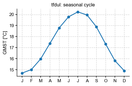
case.load('TS', period='climo')
gm = case.ds['TS'].x.da.x.gm - 273.15

fig, ax = plt.subplots(figsize=(5, 3))
ax.plot(gm.time, gm, marker='o')
ax.set_xticks(range(1, 13), list('JFMAMJJASOND'))
ax.set_ylabel('GMST [°C]')
ax.set_title(f'{case.casename}: seasonal cycle');
print('mean of the monthly climatology:', float(gm.mean()).__round__(3))

>>> case.ds["TS"] will be reloaded due to a different period/hstr.

>>> case.ds["TS"] created
mean of the monthly climatology: 17.392

case.load('PRECT', period=['djf', 'jja'])
pr = case.ds['PRECT'].x.da * 8.64e7   # m/s -> mm/day
pr.attrs['units'] = 'mm/day'
print('global mean precipitation [mm/day]:', {str(p): round(float(v), 3) for p, v in zip(pr.period.values, pr.x.gm.values)})

>>> case.ds["PRECT"] created
global mean precipitation [mm/day]: {'djf': 3.039, 'jja': 3.182}

Maps¶

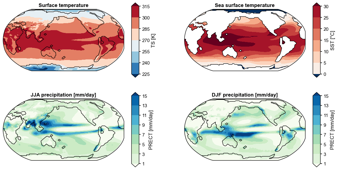
The experiments use paleogeographies, so the modern Cartopy coastlines would be wrong. Passing a sea-surface variable as ssv draws the coastlines from its land mask instead.

case.load('SST', period='ann')
sst = case.ds['SST'].x.da

fig, axs = plt.subplots(2, 2, figsize=(14, 7), subplot_kw={'projection': ccrs.Robinson(central_longitude=180)})
axs = axs.ravel()
ts.x.plot(ax=axs[0], ssv=sst)
sst.x.plot(ax=axs[1])
pr.sel(period='jja').x.plot(ax=axs[2], ssv=sst, title='JJA precipitation [mm/day]', cmap='GnBu', levels=np.arange(1, 17, 2))
pr.sel(period='djf').x.plot(ax=axs[3], ssv=sst, title='DJF precipitation [mm/day]', cmap='GnBu', levels=np.arange(1, 17, 2));

>>> case.ds["SST"] created

Pressure-level fields¶

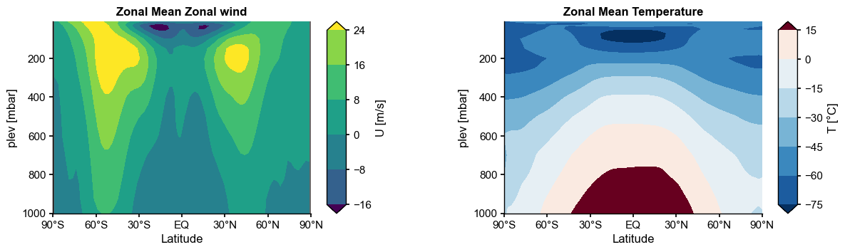
The 3-D atmosphere fields are already on 17 pressure levels (dim plev, hPa), so no get_plev step is needed. HadCM3 uses an Arakawa B-grid: winds sit on a 96 × 72 grid offset from the 96 × 73 temperature grid. Each loaded variable keeps its native grid, with an area weight that matches it.

case.load('U', period='ann')
case.load('T', period='ann')
print('U:', dict(case.ds['U'].x.da.sizes), '| T:', dict(case.ds['T'].x.da.sizes))

t_zm = case.ds['T'].x.da.x.zm - 273.15
t_zm.attrs['units'] = '°C'

fig, axs = plt.subplots(1, 2, figsize=(14, 3.5), gridspec_kw={'wspace': 0.4})
case.ds['U'].x.da.x.zm.x.plot(ax=axs[0])
t_zm.x.plot(ax=axs[1], title='Zonal Mean Temperature')
for ax in axs: ax.invert_yaxis()

>>> case.ds["U"] created
>>> case.ds["T"] created
U: {'plev': 17, 'lat': 72, 'lon': 96} | T: {'plev': 17, 'lat': 73, 'lon': 96}

Derived variables¶

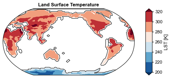
load checks the registry in x4c.diags for names that are not in the files. A name the model writes directly wins: HadCM3 has PRECT, so the CESM recipe (PRECC + PRECL) is not used. Recipes built from names the spec translates do run. LST is TS masked by LANDFRAC > 0.5, two variables that come from different HadCM3 files.

case.load('LST', period='jja')
lst = case.ds['LST']
print(f'JJA global-mean land surface temperature: {float(lst.x.gm) - 273.15:.2f} °C')
lst.x.plot(ssv=sst, cyclic=True);

>>> LST is a supported derived variable.
>>> case.ds["TS"] will be reloaded due to a different period/hstr.
>>> case.ds["TS"] created
>>> case.ds["LANDFRAC"] created
>>> case.ds["LST"] created
JJA global-mean land surface temperature: 18.60 °C

Spells¶

case.calc works too. Leave the annualization field empty (vn::sa_method), since the data are already time means, and pass period through.

print(case.calc('GMST ~ TS::gm', period='climo', verbose=False).values.round(2))
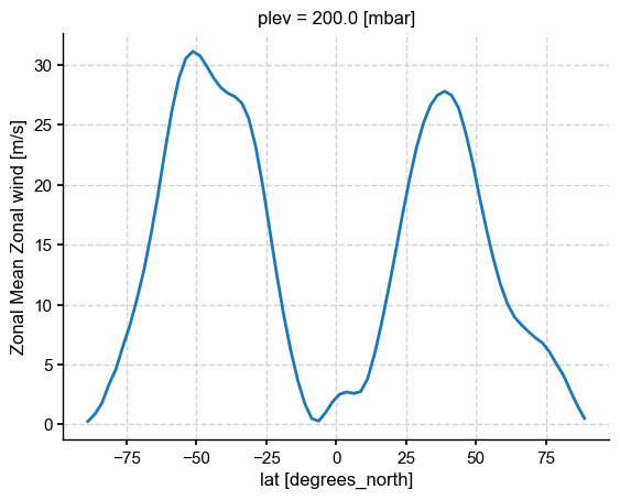
case.calc('U200 ~ U.sel(plev=200)::zm', period='ann', verbose=False).plot();

[14.69 15.01 15.97 17.38 18.78 19.78 20.23 19.95 18.88 17.32 15.81 14.91]

Raw names and `hstr`¶

Any raw source name can be loaded as well. When a name exists in more than one file group, hstr picks the group. The isotope tracer fields are deliberately left out of the translation table, because their meaning has not been confirmed yet (see spec.notes above).

try:
    case.load('temp_mm_srf', period='ann')
except ValueError as e:
    print('ValueError:', e)

case.load('q_mm_hyb', period='ann', hstr='isotope_and_atmos_clomun_data')
print(dict(case.ds['q_mm_hyb'].x.da.sizes))

ValueError: `temp_mm_srf` exists in several hstr ['isotope_and_atmos_clomun_data', 'precip_temp_shum_msl_surf_data']; pass `hstr=`.
>>> case.ds["q_mm_hyb"] created
{'lev': 19, 'lat': 73, 'lon': 96}

Extending the translation table¶

vn_dict entries are merged over the model’s own table, so names can be added or redefined for one case without touching the built-in spec. A value is a source name, or a dict with src, hstr, scale, offset, units, long_name, comp and isel.

case2 = x4c.Timeseries(
    f'{root}/tfdul', model='hadcm3',
    vn_dict={
        'TSC': {'src': 'temp_mm_srf', 'hstr': 'precip_temp_shum_msl_surf_data',
                'offset': -273.15, 'units': '°C', 'long_name': 'Surface temperature'},
        'PRECT_mmday': {'src': 'precip_mm_srf', 'scale': 86400, 'units': 'mm/day'},
    },
)
case2.load('TSC', period='ann', verbose=False)
case2.load('PRECT_mmday', period='ann', verbose=False)
print(f"TSC gm = {float(case2.ds['TSC'].x.da.x.gm):.2f} °C, PRECT_mmday gm = {float(case2.ds['PRECT_mmday'].x.da.x.gm):.3f} mm/day")

>>> case.root_dir: /glade/campaign/univ/umcp0052/data/iHadCM3/Data/tfdul
>>> case.model: hadcm3
>>> case.path_pattern: ['{case}.{period}_{hstr}.nc', '{case}.{hstr}.nc']
>>> case.casename: tfdul
>>> 54 files indexed; case.vns[hstr] created for hstr: ['SST_Seaice_data', 'isotope_and_atmos_clomun_data', 'precip_temp_shum_msl_surf_data', 'qrfrac.type', 'qrparm.mask', 'qrparm.orog']
>>> periods: ['jan', 'feb', 'mar', 'apr', 'may', 'jun', 'jul', 'aug', 'sep', 'oct', 'nov', 'dec', 'djf', 'mam', 'jja', 'son', 'ann']
>>> Skipping file matching no path pattern: tfdul_isotope_and_atmos_clomun_data.nc
TSC gm = 17.39 °C, PRECT_mmday gm = 3.091 mm/day

Across experiments¶

Because every case is read the same way, comparing all 25 experiments is a loop. Five of them hold only the boundary-condition files; LANDFRAC still loads for those.

import contextlib, io

rows = []
for expt in expts:
    with contextlib.redirect_stdout(io.StringIO()):   # silence the per-case index banner
        c = x4c.Timeseries(f'{root}/{expt}', model='hadcm3')
    row = {'expt': expt}
    c.load('LANDFRAC', verbose=False)
    row['land fraction'] = float(c.ds['LANDFRAC'].x.da.x.gm)
    if c.reader.has('TS'):
        c.load('TS', period='ann', verbose=False)
        c.load('PRECT', period='ann', verbose=False)
        row['GMST [°C]'] = float(c.ds['TS'].x.da.x.gm) - 273.15
        row['precip [mm/day]'] = float(c.ds['PRECT'].x.da.x.gm) * 8.64e7
    rows.append(row)

df = pd.DataFrame(rows).set_index('expt')
df.round(3)

d = df.dropna()
fig, ax = plt.subplots(figsize=(5, 4))
ax.scatter(d['GMST [°C]'], d['precip [mm/day]'])
for name, r in d.iterrows():
    ax.annotate(name, (r['GMST [°C]'], r['precip [mm/day]']), fontsize=8, xytext=(3, 3), textcoords='offset points')
ax.set_xlabel('GMST [°C]')
ax.set_ylabel('Global-mean precipitation [mm/day]');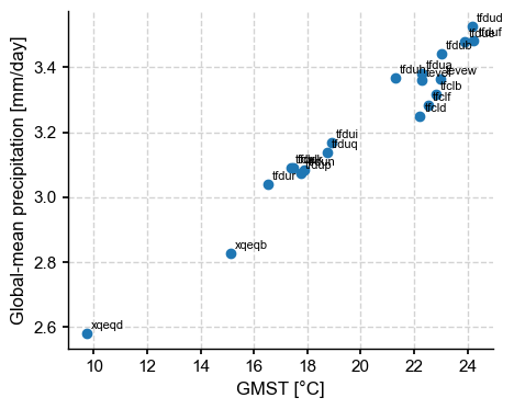

Adding another model¶

Another model needs only a spec, either inline as Timeseries arguments or registered once with x4c.models.register(x4c.models.ModelSpec(...)) and then selected by model=. For example, a CMIP-style layout with one variable per file:

case = x4c.Timeseries(
    '/path/to/run1',
    path_pattern='{vn}_Amon_{case}_{timespan}.nc',
    vn_dict={'TREFHT': 'tas', 'PRECT': {'src': 'pr', 'scale': 1e-3, 'units': 'm/s'}},
    dim_map={'latitude': 'lat', 'longitude': 'lon'},
)
case.load('TREFHT')   # all timespans concatenated along time

Caveats¶

About the iHadCM3 data

Climatologies, not time series. Every file is a multi-year mean with one time step. Its time units (e.g. days since 13850-12-00) are not valid CF, so times are not decoded and the time dim is dropped. Anything that needs a real time axis, such as .x.annualize(), the ann field of a spell, or .x.anom, does not apply here. Use period= instead.
Isotope tracers are untranslated. The stash-coded fields in the isotope file (q_mm_hyb, q_mm_hyb_1, the snowdepth_mm_srf* / icedepth_mm_srf* pairs) carry CF and PCMDI names that the conversion tool (xconv) guessed from the default STASHmaster; ignore them. Their meaning was inferred only from value ratios (see spec.notes), so confirm it with the data provider before use. In that file, temp_mm_srf and temp_mm_srf_1 are not surface temperature. No precipitation isotopes or hybrid-level H₂¹⁶O are present, so δ¹⁸O of precipitation cannot be computed from these files alone.
Incomplete experiments. tfduc, tfdug, tfduj, tfdum and tfduo hold only the boundary-condition files. <expid>_isotope_and_atmos_clomun_data.nc (no period) is a copy of the SON file and is skipped.
Native B-grid. Winds and their transports (U, V, OMEGA, Q, UQ, VQ) are on the 96 × 72 velocity grid; temperature-point fields are on 96 × 73. Arithmetic that mixes the two grids (e.g. U * T) needs one of them interpolated first.
SST is the top ocean level (5 m) of potential temperature. PRECT is converted from kg m⁻² s⁻¹ (mislabelled kg m-2 in the files) to CESM’s m/s.

About the mechanism

Methods that need the CESM layout. case.plot, case.quickview, case.get_ts and case.save_means raise NotImplementedError for a spec-driven case. load, calc and the .x accessors are the supported path.
calc caches by spell text only. Calling case.calc('TS::gm', period='jan') and then the same spell with period='jul' returns the January result. Pass recalculate=True or use a distinct alias ('TS_jul ~ TS::gm').
load replaces the cached variable. Loading TS with a new period replaces case.ds['TS'], and a derived variable such as LST reloads its inputs for its own period.
hstr precedence. A vn_dict entry that names its hstr always uses it. The hstr= argument of load only picks the file group for raw names that appear in several.
Variable listing. The raw names of a file group are read from its first file, so all files in a group are assumed to hold the same variables.
Curvilinear grids load, but the area weight is cos(lat) rather than the true cell area, and .x.plot cannot draw them without regridding first.
Plotting. Pressure-level cross-sections are drawn with pressure increasing upward; call ax.invert_yaxis(). A known cartopy/shapely bug makes .x.plot raise GEOSException when explicit levels start exactly at the field’s minimum (e.g. precipitation = 0), so start the levels just above it.