Sea surface height from the MESACLIP historical run

Run this notebook interactively on CIRRUS BinderHub.

Sea surface height from MESACLIP¶

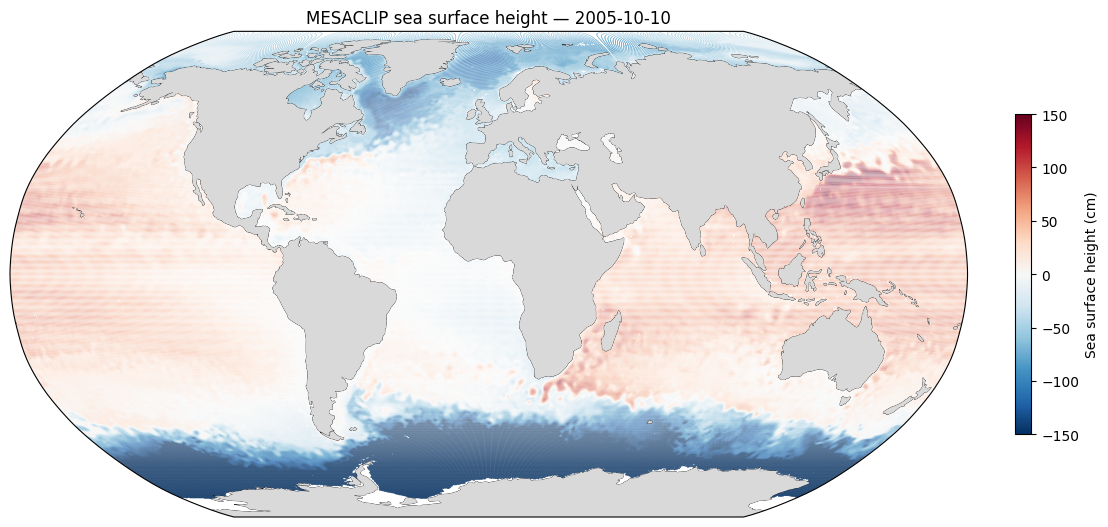
This is a minimal example: open the MESACLIP high-resolution (0.1° ocean) CESM iHESP historical simulation from GDEX and plot a single day of sea surface height. For a fuller workflow — regridding to a regular grid and building an interactive map — see the companion notebook MESACLIP SST regridding.

The data is served as a kerchunk reference over the underlying model output, so one xr.open_dataset(..., engine="kerchunk") call exposes the whole daily record as a virtual xarray.Dataset.

import os
import xarray as xr
import matplotlib.pyplot as plt
import cartopy.crs as ccrs
import cartopy.feature as cfeature
import numpy as np
import cftime

# Auto-select the kerchunk reference: POSIX where /gdex/data is mounted (NCAR
# HPC, CIRRUS Binder), otherwise the OSDF reference over the network.
posix_ref = "/gdex/data/d651007/kerchunk/b.e13.BHISTC5.ne120_t12.cesm-ihesp-hires1.0.46-1920-2005.010.ocn.day_1.parq"
store = posix_ref if os.path.exists(posix_ref) else "https://data.gdex.ucar.edu/d651007/kerchunk/b.e13.BHISTC5.ne120_t12.cesm-ihesp-hires1.0.46-1920-2005.010.ocn.day_1-remote-osdf.parq"
print(store)

ds = xr.open_dataset(store, engine="kerchunk", decode_timedelta=False, chunks={})
ds

Loading...

The sea-surface-height field is SSH_2 (long name “Sea Surface Height”, units cm) on the model’s 0.1° tripole grid, with 2D geographic coordinates TLAT/TLONG. We pull one day and its grid — everything else stays lazy.

# CESM uses a no-leap (365-day) calendar, so time is a cftime index, not datetime64.
# Select with a matching cftime object rather than a string.
target = cftime.DatetimeNoLeap(2005, 10, 10)
day = ds["SSH_2"].sel(time=target, method="nearest").load()   # cm
lat = ds["TLAT"].isel(time=0).load()
lon = ds["TLONG"].isel(time=0).load()
day

Loading...

# Subsample for a light global plot, and use scatter (one point per cell) rather than pcolormesh. 
c  = 4
z  = day.values[::c, ::c]
la = lat.values[::c, ::c]
lo = ((lon.values[::c, ::c] + 180) % 360) - 180     # 0–360 → −180..180
m  = np.isfinite(z)                                  # drop land (NaN)

fig, ax = plt.subplots(figsize=(11, 5.5), subplot_kw={"projection": ccrs.Robinson()},
                       constrained_layout=True)
sc = ax.scatter(lo[m], la[m], c=z[m], s=1.2, marker=".", linewidths=0,
                cmap="RdBu_r", vmin=-150, vmax=150, transform=ccrs.PlateCarree())
ax.add_feature(cfeature.LAND, facecolor="0.85", zorder=2)
ax.coastlines(linewidth=0.4)
ax.set_global()
plt.colorbar(sc, ax=ax, shrink=0.6, label="Sea surface height (cm)")
ax.set_title(f"MESACLIP sea surface height — {day.time.dt.strftime('%Y-%m-%d').item()}")
plt.show()