This notebook is adapted from the NCAR gallery in the Pangeo collection
Introduction
Input Data Access
This notebook illustrates how to compute surface ocean heat content using potential temperature data from CESM2 Large Ensemble Dataset (https://
www .cesm .ucar .edu /community -projects /lens2) hosted on NCAR’s GDEX.
# Imports
import intake
import numpy as np
import pandas as pd
import xarray as xr
import seaborn as sns
import re
import os
import matplotlib.pyplot as plt
import cf_units as cf
import os
import dask
from dask_jobqueue import PBSCluster
import shutil
from dask.distributed import Client, LocalCluster
from dask.distributed import performance_reportinit_year0 = '1991'
init_year1 = '2020'
final_year0 = '2071'
final_year1 = '2100'def to_daily(ds):
year = ds.time.dt.year
day = ds.time.dt.dayofyear
# assign new coords
ds = ds.assign_coords(year=("time", year.data), day=("time", day.data))
# reshape the array to (..., "day", "year")
return ds.set_index(time=("year", "day")).unstack("time")# Set up your sratch folder path
username = os.environ["USER"]
glade_scratch = "/glade/derecho/scratch/" + username
print(glade_scratch)
#
/glade/derecho/scratch/harshah
# Auto-select the intake-ESM catalog: POSIX where /gdex/data is mounted (NCAR
# HPC, CIRRUS Binder), otherwise the OSDF catalog over the network.
posix_catalog = "/gdex/data/d010092/catalogs/d010092-posix.json"
catalog_url = posix_catalog if os.path.exists(posix_catalog) else "https://osdata.gdex.ucar.edu/d010092/catalogs/d010092-osdf.json"
print(catalog_url)
Set up Dask Cluster
Setting up a dask cluster
Since we plan to run this noteook on NCAR’s HPC i.e, Casper, we will use a PBS Scheduler
def get_pbs_cluster(n_workers=5):
    """PBSCluster on NCAR HPC (Casper/Derecho)."""
    scratch = f"/glade/derecho/scratch/{os.environ.get('USER', '')}"
    cluster = PBSCluster(
        job_name        = "dask-wk24-hpc",
        cores           = 1,
        memory          = "8GiB",
        processes       = 1,
        local_directory = f"{scratch}/dask/spill/",
        log_directory   = f"{scratch}/dask/logs/",
        resource_spec   = "select=1:ncpus=1:mem=8GB",
        queue           = "casper",
        walltime        = "5:00:00",
        interface       = "ext",
    )
    cluster.scale(n_workers)
    return cluster


def get_local_cluster():
    """LocalCluster for a laptop or a CIRRUS Binder pod (no PBS scheduler)."""
return LocalCluster()# Auto-detect the environment: a `qsub` on PATH means a PBS scheduler is present
# (Casper/Derecho) -> PBSCluster; otherwise fall back to LocalCluster (CIRRUS
# Binder or a laptop). No editing needed to move between environments.
on_hpc = bool(shutil.which("qsub"))
cluster = get_pbs_cluster() if on_hpc else get_local_cluster()
client = Client(cluster)
if on_hpc:
client.wait_for_workers(n_workers=5)
print(f"Detected {'NCAR HPC -> PBSCluster' if on_hpc else 'no PBS -> LocalCluster'}")
clusterData Loading
Load CESM2 LENS zarr data from GDEX using an intake-ESM catalog
For more details regarding the dataset. See, https://
gdex .ucar .edu /datasets /d010092 /#
cesm_cat = intake.open_esm_datastore(catalog_url)
cesm_cat# cesm_cat.df['variable'].valuescesm_temp = cesm_cat.search(variable ='TEMP', frequency ='monthly',experiment='historical')
cesm_tempcesm_temp.df['path'].values<ArrowExtensionArray>
['osdf:///ncar-gdex/d010092/ocn/monthly/cesm2LE-historical-cmip6-TEMP.zarr']
Length: 1, dtype: large_string[pyarrow]dsets_cesm = cesm_temp.to_dataset_dict(xarray_open_kwargs={'engine':'zarr','backend_kwargs':{'consolidated': True,'zarr_format': 2}})
--> The keys in the returned dictionary of datasets are constructed as follows:
	'component.experiment.frequency.forcing_variant'
cesm_temp.keys()['ocn.historical.monthly.cmip6']historical = dsets_cesm['ocn.historical.monthly.cmip6']
# future_smbb = dsets_cesm['ocn.ssp370.monthly.smbb']
# future_cmip6 = dsets_cesm['ocn.ssp370.monthly.cmip6']# %%time
# merge_ds_cmip6 = xr.concat([historical, future_cmip6], dim='time')
# merge_ds_cmip6 = merge_ds_cmip6.dropna(dim='member_id')historicalChange units
orig_units = cf.Unit(historical.z_t.attrs['units'])
orig_unitsUnit('centimeters')def change_units(ds, variable_str, variable_bounds_str, target_unit_str):
orig_units = cf.Unit(ds[variable_str].attrs['units'])
target_units = cf.Unit(target_unit_str)
variable_in_new_units = xr.apply_ufunc(orig_units.convert, ds[variable_bounds_str], target_units, dask='parallelized', output_dtypes=[ds[variable_bounds_str].dtype])
return variable_in_new_unitshistorical['z_t']depth_levels_in_m = change_units(historical, 'z_t', 'z_t', 'm')
hist_temp_in_degK = change_units(historical, 'TEMP', 'TEMP', 'degK')
# fut_cmip6_temp_in_degK = change_units(future_cmip6, 'TEMP', 'TEMP', 'degK')
# fut_smbb_temp_in_degK = change_units(future_smbb, 'TEMP', 'TEMP', 'degK')
#
hist_temp_in_degK = hist_temp_in_degK.assign_coords(z_t=("z_t", depth_levels_in_m['z_t'].data))
hist_temp_in_degK["z_t"].attrs["units"] = "m"
hist_temp_in_degKdepth_levels_in_m.isel(z_t=slice(0, -1))#Compute depth level deltas using z_t levels
depth_level_deltas = depth_levels_in_m.isel(z_t=slice(1, None)).values - depth_levels_in_m.isel(z_t=slice(0, -1)).values
# Optionally, if you want to keep it as an xarray DataArray, re-wrap the result
depth_level_deltas = xr.DataArray(depth_level_deltas, dims=["z_t"], coords={"z_t": depth_levels_in_m.z_t.isel(z_t=slice(0, -1))})
depth_level_deltas Data Analysis
Compute Ocean Heat content for ocean surface
Ocean surface is considered to be the top 100m
The formula for this is:
Where H is ocean heat content, the value we are trying to calculate,
is the density of sea water, ,
is the specific heat of sea water, ,
is the depth limit of the calculation in meters,
and is the temperature at each depth in degrees Kelvin.
def calc_ocean_heat(delta_level, temperature):
    rho = 1026 #kg/m^3
    c_p = 3990 #J/(kg K)
    weighted_temperature = delta_level * temperature
    heat = weighted_temperature.sum(dim="z_t")*rho*c_p
    return heat
# Remember that the coordinate z_t still has values in cm
hist_temp_ocean_surface = hist_temp_in_degK.where(hist_temp_in_degK['z_t'] < 1e4,drop=True)
hist_temp_ocean_surfacedepth_level_deltas_surface = depth_level_deltas.where(depth_level_deltas['z_t'] <1e4, drop= True)
depth_level_deltas_surfacehist_ocean_heat = calc_ocean_heat(depth_level_deltas_surface,hist_temp_ocean_surface)
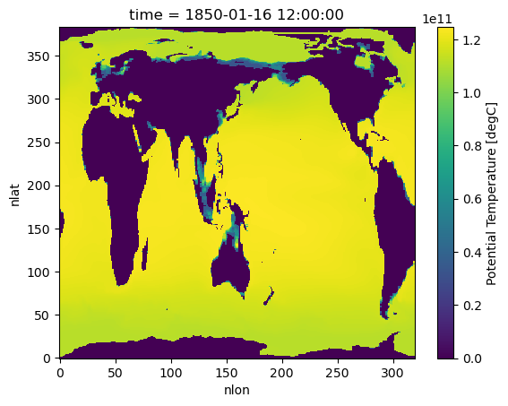
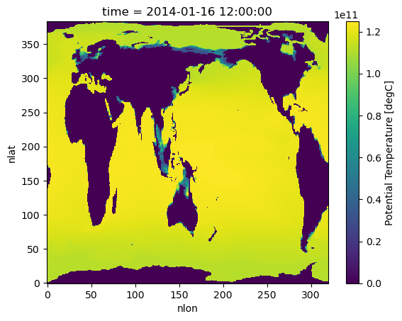
hist_ocean_heatPlot Ocean Heat
%%time
# Jan, 1850 average over all memebers
# hist_ocean_avgheat = hist_ocean_heat.mean('member_id')
hist_ocean_avgheat = hist_ocean_heat.isel({'time':[0,-12]}).mean('member_id')
hist_ocean_avgheat
CPU times: user 39.6 ms, sys: 3.67 ms, total: 43.3 ms
Wall time: 42.9 ms
%%time
hist_ocean_avgheat.isel(time=0).plot()
/glade/u/home/harshah/.conda/envs/osdf/lib/python3.11/site-packages/distributed/client.py:3375: UserWarning: Sending large graph of size 14.27 MiB.
This may cause some slowdown.
Consider loading the data with Dask directly
or using futures or delayed objects to embed the data into the graph without repetition.
See also https://docs.dask.org/en/stable/best-practices.html#load-data-with-dask for more information.
warnings.warn(
CPU times: user 11.5 s, sys: 687 ms, total: 12.2 s
Wall time: 1min 30s
%%time
#Plot ocean heat for Jan 2014
hist_ocean_avgheat.isel(time=1).plot()
CPU times: user 11.5 s, sys: 455 ms, total: 12 s
Wall time: 1min 3s
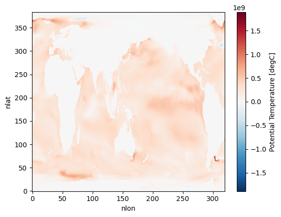
Has the surface ocean heat content increased with time for January ? (Due to Global Warming!)
hist_ocean_avgheat_ano = hist_ocean_avgheat.isel(time=1) - hist_ocean_avgheat.isel(time=0)%%time
hist_ocean_avgheat_ano.plot()/glade/u/home/harshah/.conda/envs/osdf/lib/python3.11/site-packages/distributed/client.py:3375: UserWarning: Sending large graph of size 14.27 MiB.
This may cause some slowdown.
Consider loading the data with Dask directly
or using futures or delayed objects to embed the data into the graph without repetition.
See also https://docs.dask.org/en/stable/best-practices.html#load-data-with-dask for more information.
warnings.warn(
CPU times: user 10.9 s, sys: 344 ms, total: 11.2 s
Wall time: 1min 1s
cluster.close()