Chapter 4: Understanding GCM climate change modeling and attributes, strengths, limitations

This Chapter provides an overview and guidance on the following topics:

• Introduction to the Intergovernmental Panel on Climate Change (IPCC), The Coupled Model Intercomparison Projects (CMIP), the National Climate Assessments (NCA), and other institutions and institutional arrangements that provide climate-change-relevant information for North America.

• Overview of how GCMs are utilized under the IPCC framework

• Some of the limitations and challenges of GCMs: current strengths and abilities and ongoing challenges

• Resources where GCM-derived future climate change outputs can be found for future applications

Table of Contents

• Introduction

• Goals of IPCC, CMIPs

• What do climate projections (IPCC scenarios) mean and their assumptions

• Key takeaways from the chapter

• References

Chapter 4 Key Takeaways

Summary of GCM Attributes, Strengths, and Limitations

ATTRIBUTES	STRENGTHS	LIMITATIONS
The predominant tool for advancing our understanding of climate dynamics and informing global response strategies and policy-making in addressing the challenges of climate change.	Provides Projections of Future Climate Conditions and Support for International Climate Assessments	Their accuracy depends on the quality of input data, the precision of mathematical formulations, and the computing power available that constrains the temporal and spatial resolution of the calculations.
Offer the only practical way to integrate highly non-linear systems (or system of systems) and then provide insights into their interactions.	Provides an Understanding of Climate Processes and Evaluation of Climate Change Impacts	There is inherent uncertainty in modeling complex systems, which means that they cannot predict exact outcomes.
Allows for Testing Hypotheses and Development of Mitigation and Adaptation Strategies	The ability to reproduce the temporal evolution of the climate system has strengthened our confidence in properly contrasting the changes between different societal emission pathways.	Uncertainties remain regarding climate models’ ability to represent some aspects of the earth-climate system (aersol-cloud interactions, ice sheet dynamics, carbon cycle feedback loops, AI, ground truthing)
Provides (and continue to improve upon) representation of climate variability across a broad range timescales.	The spatial skill of models in reproducing the observed patterns continues to improve with temperature historically already well represented, and precipitation gradually improving.	While some of the differences in climate modeling results have decreased over time; others have increased.
		The lack of constraints on the GCMs over the historic period is in contrast to how these same GCMs might be used to produce reanalysis data sets over the historic period, where model states are continually brought back to be consistent to observations collected over the period.

Attribution

Much of the material and images used in this chapter are derived from the following MetEd Lessons: Introduction to Climate Models; Preparing Hydro-climate Inputs for Climate Change in Water Resource Planning. The source of this material is the COMET® Website at http://meted.ucar.edu/ of the University Corporation for Atmospheric Research (UCAR), sponsored in part through cooperative agreement(s) with the National Oceanic and Atmospheric Administration (NOAA), U.S. Department of Commerce (DOC). ©1997-2024 University Corporation for Atmospheric Research. All Rights Reserved.

4.1 Introduction

This chapter provides an overview of General Circulation Models (GCMs), also known as Global Climate Models, and how they are employed within the international research consortia providing research and data relevant for understanding and characterizing the impacts of climate change. In this chapter, we provide an overview of the strengths and weaknesses of GCMs, which are the fundamental tools used in climate science to provide insights into our understanding of climate change. These sophisticated computer models simulate the Earth’s climate systems, including the atmosphere, oceans, land surface, and ice, enabling an accounting of the energy storage and energy fluxes into and out of the earth system.

Here are some key benefits of GCMs to climate-change understanding.

Provides Projections of Future Climate Conditions and Support for International Climate Assessments

GCMs enable scientists to project future climate conditions under various scenarios, such as those outlined in the IPCC SRES, RCP, and SSP frameworks (which we discuss further below). By inputting different concentrations of greenhouse gases, GCMs can simulate how the climate might change in the future and provide the scientific basis for the climate projections and policies discussed in IPCC reports, helping to inform policymakers, businesses, and the public about potential risks and necessary adaptations.

Provides an Understanding of Climate Processes and Evaluation of Climate Change Impacts

GCMs simulate the complex interactions between different components of the Earth’s climate system. This helps scientists understand fundamental processes such as the water cycle, energy balance, and atmospheric dynamics. By modeling these processes, GCMs provide insights into how changes in one part of the system (like increased atmospheric CO2) can affect other parts (like global temperature and precipitation patterns). This in turn, helps assess potential impacts of climate change on various sectors, including agriculture, water resources, and health. For instance, models can project changes in rainfall patterns, heat waves, and the frequency of extreme weather events, which are crucial for planning and mitigation strategies in vulnerable regions.

Allows for Testing Hypotheses and Development of Mitigation and Adaptation Strategies

GCMs are valuable for testing scientific hypotheses about the climate system. By altering specific variables or processes within the model, researchers can explore how these changes affect climate outcomes, thereby testing our understanding of climate mechanisms and feedbacks, and contributing to detection and attribution studies (discussed in Chapter 3). This also allows researchers to simulate different future climate scenarios in developing effective climate-change mitigation and adaptation strategies, such as emission reductions, reforestation, and technological innovations including geoengineering, in curbing climate impacts.

While GCMs are invaluable, they do come with limitations. Their accuracy depends on the quality of input data, the precision of mathematical formulations, and the computing power available that constrains the temporal and spatial resolution of the calculations. Moreover, there is inherent uncertainty in modeling complex systems, which means that while GCMs are excellent for exploring possible futures, they cannot predict exact outcomes, an issue we will discuss further in this chapter, including the discussion of ensembles. Despite these challenges, GCMs are still the predominant tool for advancing our understanding of climate dynamics and informing global response strategies and policy-making in addressing the challenges of climate change.

Further below we provide a broader introduction to the climate modeling process.

To learn more about climate models visit Introduction Introduction to Climate Models

4.2 Goals of the IPCC, CMIPs, NCA

4.2.1 IPCC

The Intergovernmental Panel on Climate Change (IPCC) is the United Nations body tasked with assessing the science related to climate change, with its objective to provide governments at all levels with the scientific information that they can use to formulate climate policies. The assessments are provided regularly (approximately every 5-7 years), with IPCC Reports being one of the primary modalities, covering the scientific basis of climate change, its impacts and future risks, and options for adaptation and mitigation.

The IPCC’s primary goals

Assess Scientific Information

in its assessment reports through comprehensive reviews of the latest scientific literature on climate change, its impacts, and potential future risks, involving synthesizing findings from thousands of scientific studies; and special reports on specific aspects of climate change as requested by the IPCC member governments, addressing emerging issues or areas requiring detailed examination.

Evaluate Climate Change Impacts and Risks

on global and regional scales by sssessing the observed and projected impacts of climate change on natural and human systems at both global and regional scales. This includes examining effects on ecosystems, weather patterns, sea levels, and human health. And provide risk analyses by Analyzing the risks associated with different levels of global warming, providing insights into the potential consequences of various climate change scenarios.

Inform Policymakers

with scientific information that is policy-relevant but not policy-prescriptive. This means offering evidence-based findings without advocating for specific policies. Also provides Summaries for Policymakers that distill the key findings of comprehensive reports into actionable information for decision-makers.

Support International Climate Negotiations

such as providing scientific assessments that support the United Nations Framework Convention on Climate Change and international climate negotiations. IPCC reports are often used as the scientific basis for global climate agreements and negotiations, such as the Paris Agreement.

Assess Mitigation and Adaptation Strategies

Evaluate strategies for reducing greenhouse gas emissions and enhancing carbon sinks. This includes assessing the potential of renewable energy, energy efficiency, carbon capture and storage, and other mitigation technologies. And assess strategies for adapting to the impacts of climate change. This includes evaluating measures to increase resilience in agriculture, water resources, infrastructure, and public health.

Note that the IPCC’s goals, as stated above, do not explicitly include the mandate of providing future-change model outputs and datasets that would be useful, say, for this primer’s user audience (aka needed to drive more local-scale impact models). However, Section Learn More provides resources where many of these data, including CMIP6 [discussed below] and other data, can be found.

4.2.2 CMIP

The Coupled Model Intercomparison Project (CMIP) is a collaborative framework designed to synthesize climate-modeling efforts from a number of weather and climate centers to improve knowledge of past, present, and future climate change from natural variability or in response to anthropogenic changes to radiative forcing [1]. CMIP is under the Working Group on Coupled Modelling (WGCM) of the World Climate Research Programme (WCRP), with the latter under the joint sponsorship of the World Meteorological Organization (WMO) and the International Council for Science (ISCU). In terms of the CMIP acronym, “Coupled” refers to the interconnected components of the climate system (e.g., land, air, water, etc.) that are simulated by the climate models; “intercomparison” references the many models that are available to compare with observations and to one another to characterize model uncertainty and scenario uncertainty. The CMIP project started in 1995 and has multiple versions of generated datasets, including CMIP3 (2005), CMIP5 (2011) (there was no CMIP4), and CMIP6 (2018), with the members of the CMIP Core Panel currently working on the design of CMIP7.

Important goals of CMIP

• Standardize global climate model (GCM) experiments and model output

• Compare and evaluate GCMs used in the climate studies`

• Make the CMIP GCM data publicly available

4.2.3 CORDEX

One notable model intercomparison project under the umbrella of CMIP is the COordinated Regional Climate Down-scaling Experiment or CORDEX (Gutowski et al. 2016), for comparing and evaluating regional dynamical and statistical downscaling techniques and their appropriateness for climate services. This project has helped to coordinate higher-resolution regional modeling studies for different regions around the world. This experiment complements and adds value to the CMIP global models, particularly in complex topography zones, coastal areas and small islands, as well as for extremes.

4.2.4 NCA

The National Climate Assessment (NCA) is a key initiative of the U.S. Global Change Research Program (USGCRP) and is aimed at assessing and summarizing the impacts of climate change on the country and involves contributions from hundreds of experts across various sectors. The Global Change Research Act of 1990 mandates that the USGCRP deliver a report to Congress and the President not less frequently than every four years that “integrates, evaluates, and interprets the findings of the Program and discusses the scientific uncertainties associated with such findings; analyzes the effects of global change on the natural environment, agriculture, energy production and use, land and water resources, transportation, human health and welfare, human social systems, and biological diversity; and analyzes current trends in global change, both human-induced and natural, and projects major trends for the subsequent 25 to 100 years.”

The main goals of the National Climate Assessment

Inform policy guidance and resource-management decision-making

by providing policy-neutral and policy-relevant information accessible and actionable.

Enhance Public Awareness and Understanding

about the causes, impacts, and potential solutions to climate change, aiming to make the scientific information accessible to a broad audience.

Evaluate Climate Impacts and Vulnerabilities

through Regional Assessments providing detailed assessments of climate impacts and vulnerabilities at regional scales; and Sectoral Assessments evaluating the impacts of climate change on various sectors, such as health, agriculture, water resources, energy, ecosystems, and infrastructure.

Assess Adaptation and Mitigation Strategies

assess the science of adapting to a changing climate, emissions reductions, and other efforts that together describe the US’s existing and potential response to climate change, including benefits, trade-offs, targets, limitations, and best practices (while not evaluating or recommending specific adaptation or mitigation policies).

4.3 What climate projections and IPCC climate-change scenarios mean and their assumptions

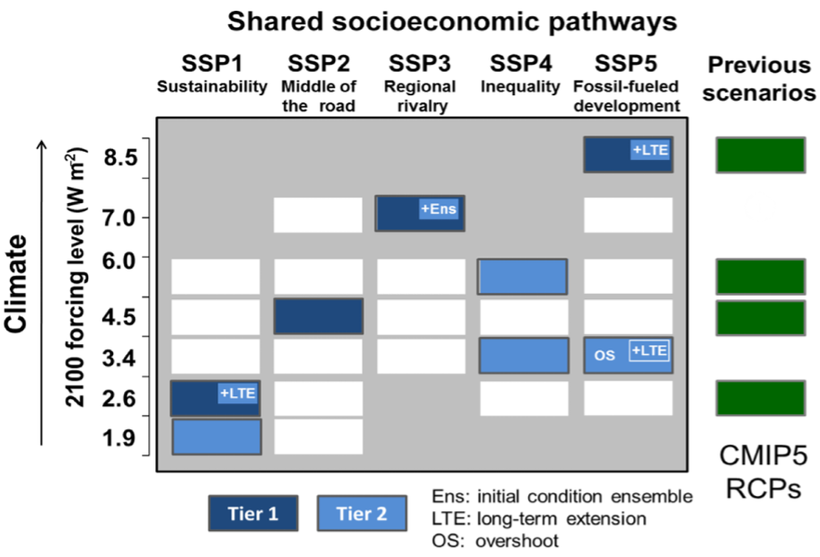
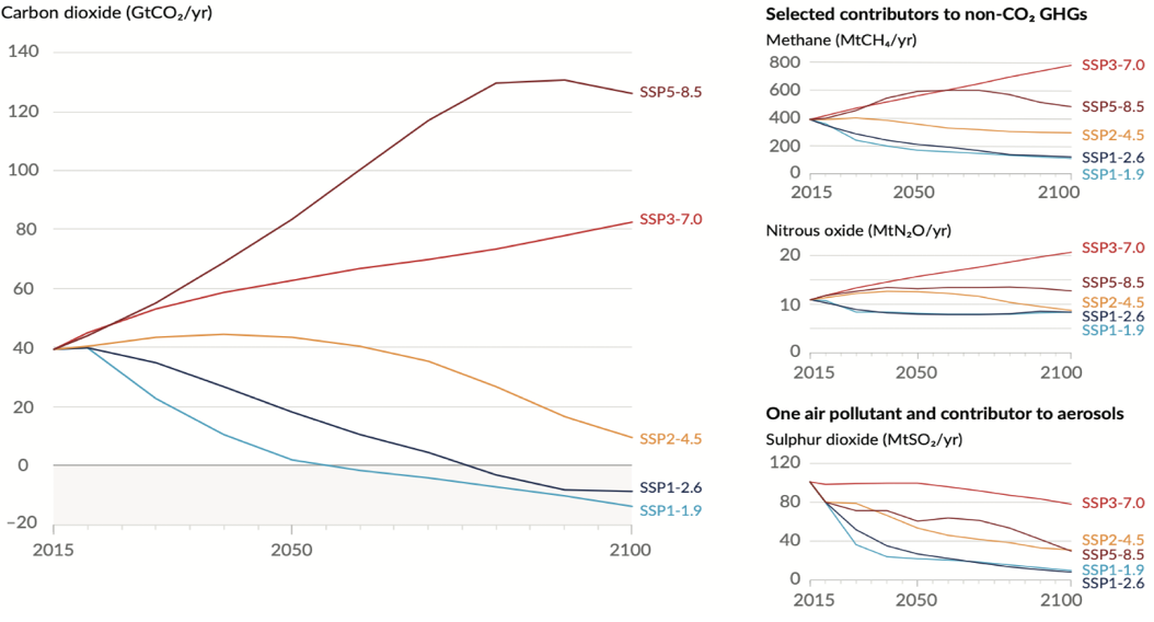
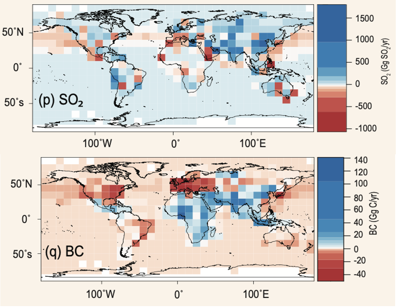
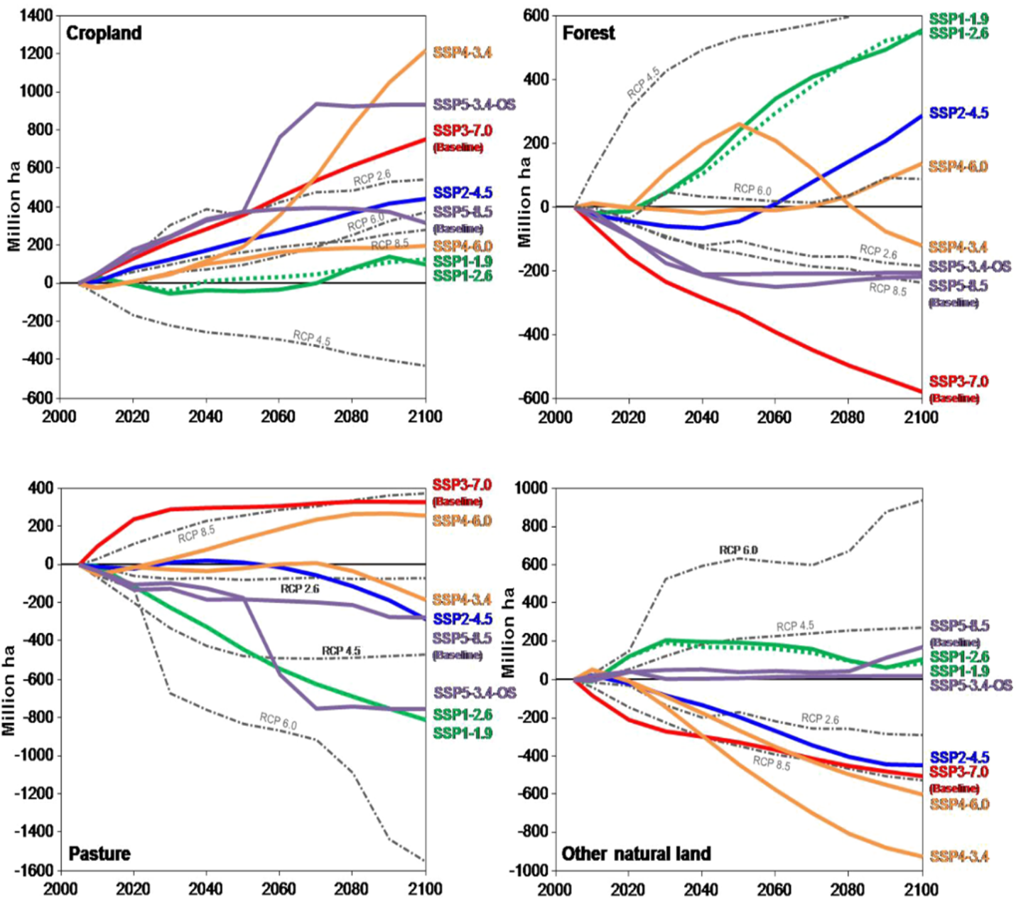
Since the early iterations of the IPCC process, a suite of coordinated experiments under the CMIP framework have been performed to offer a multi-model view of potential futures (e.g., Taylor et al. 2012). To drive the different coordinated experiments, several scenarios were developed. Over time, this process has been formalized and the initial scenarios from the Special Report on Emissions Scenarios (SRES, Nakicenovic and Swart, 2000) of CMIP3 were replaced by Representative Concentration Pathways (RCPs, Moss et al. 2010, van Vuuren et al., 2011; van Vuuren et a. 2014) of CMIP5. For the CMIP6 process (Eyring et al. 2016), a new model intercomparison project was adopted called the ScenarioMIP (O’Neill et al. 2016) in which the Shared Socio-economic Pathways, or SSPs, were presented with the goal to better understand the physical system as well as its impacts on societies. Among other improvements, this framework has helped inform the UNFCCC to formulate the Paris Agreement (IPCC 2016) with the stated objectives of limiting warming to below 2°C, or even 1.5°C (e.g., Rogelj et al. 2018). Below is a further description and comparison of these frameworks (SRES, RCPs, SSPs) developed by the IPCC community for climate modeling and assessment of future scenarios regarding greenhouse gas emissions and their impacts:

4.3.1 SRES (Special Report on Emissions Scenarios)

• Developed by: Intergovernmental Panel on Climate Change (IPCC) in 2000, and used in the IPCC’s Third and Fourth Assessment Reports.

• Purpose: To explore different scenarios of future emissions based on varying economic, social, and environmental developments without assigning likelihood to any scenario.

• Features:

  • Four narrative families (A1, A2, B1, B2) reflecting different developmental pathways.

  • Scenarios are “baseline” scenarios, they do not take into account any current or future measures to limit greenhouse gas emissions (e.g., the Kyoto Protocol).

4.3.2 RCP (Representative Concentration Pathways)

• Developed by: Introduced in the IPCC’s Fifth Assessment Report (2014).

• Purpose: To provide a set of four greenhouse gas concentration (as opposed to the SRES focus on emission inputs into the earth system) trajectories adopted by the climate-modeling community for the physical science basis of climate projections.

• Features:

  • Four pathways (RCP2.6, RCP4.5, RCP6, RCP8.5) representing different climate futures based on the radiative forcing in watts per square meter by 2100 (2.6 W/m², 4.5 W/m², etc.).

  • Includes the impact of potential future policies by considering different levels of greenhouse gas emissions and concentrations.

4.3.3 SSP (Shared Socioeconomic Pathways)

• Developed by: First used extensively in the IPCC’s Sixth Assessment Report (2021).

• Purpose: To provide a more comprehensive framework that integrates RCPs with socioeconomic factors that might influence greenhouse gas emissions.

• Features:

  • Five pathways (SSP1 through SSP5) integrating RCPs within broader narratives about socioeconomic changes, such as demographic, economic, and technological developments, intended to span the range of plausible futures, including: a world of sustainability-focused growth and equality (SSP1); a “middle of the road” world where trends broadly follow their historical patterns (SSP2); a fragmented world of “resurgent nationalism” (SSP3); a world of ever-increasing inequality (SSP4); and a world of rapid and unconstrained growth in economic output and energy use (SSP5).

  • Each SSP has different “challenges to mitigation” and “challenges to adaptation”, providing a matrix of scenarios for more refined analysis.

Further details on SSPs

The figure below presents the simple framing of the different societal storylines that form the basis of the new SSPs. At their core, they represent different societal development pathways that are describing their respective “worlds”: SSP1 sustain-ability; SSP2 middle of the road; SSP3 regional rivalry; SSP4 inequality; and SSP5 fossil-fueled development. For each of these storylines, different outcomes regarding emissions and thus concentrations of greenhouse gasses, aerosol, and land-use changes can be considered (e.g., Riahi et al., 2017). The ScenarioMIP process then performed a selection of scenarios that offer continuation to previous assessment reports. The core (Tier 1) scenarios offered to the climate-modeling communities were: SSP1-2.6, with an end-of-century radiative forcing of about 2.6 W/m²; SSP2-4.5 with 4.5 W/m²; SSP3-7.0 with 7 W/m², and SSP5-8.5 with 8.5 W/m².

Figure: SSPs from ScenarioMIP matrix with associated select forcing levels (Tier 1), from O’Neill et al., 2016.

Notable characteristics of the different SSPs are illustrated in the three figures below for well mixed global emissions; spatial emission-pattern differences between CMIP6 and CMIP5; and land-use changes over time, respectively.

Figure: Emissions of well-mixed greenhouse gases (CO2, CH4, N2O) as well as SO2. (Source: IPCC, 2021)

Figure: Spatial emissions differences between CMIP6 and the previous CMIP5 emissions for SO2 (top) and black carbon (bottom). (Source: IPCC, 2021)

Figure: Global time-series of land use changes (in million hectares) (Source: IPCC, 2021)

Modeling groups were also encouraged to perform additional experiments beyond Tier 1 scenarios. These experiments are associated with scenarios that contain reductions later in the century (so called “overshoot scenarios”) as well as a low-end emission scenario in line with the Paris Agreement (IPCC 2016): SSP1-1.9. Because of the large computational demand, most modeling centers only performed the core Tier 1 experiments. Some centers managed to simulate a large number of ensemble members for select experiments. These experiments are the CMIP6 simulations associated with the ScenarioMIP project. However, there are a total of 23 independent intercomparison projects that are part of CMIP6, and thus significantly more model output is available to study physical systems.

4.3.4 Comparison and Contrast

• Application in Climate Models: SRES scenarios were used primarily before the development of RCPs, which are now commonly used in climate modeling along with SSPs. SSPs are particularly significant for their use in exploring the impacts of socioeconomic factors on emission scenarios and vice versa.

• Policy Integration: SRES scenarios did not consider future climate policies explicitly. RCPs began to incorporate potential future policies indirectly through assumptions about radiative forcing. SSPs explicitly integrate both mitigation and adaptation challenges within their scenarios, offering a nuanced framework for policy discussions.

In summary, as climate science has advanced, so too has the complexity and applicability of these scenarios. Each successive framework has built upon the last, providing more detailed tools for understanding and addressing the multifaceted challenges of climate change.

4.4 Earth-system climate modeling – current strengths and abilities

Climate models offer the only practical way to integrate highly non-linear systems (or system of systems) and then provide insights into their interactions.

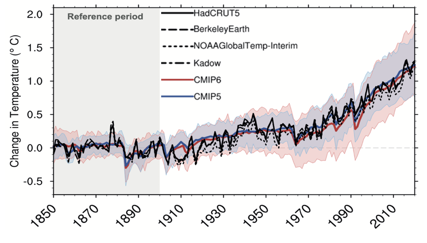
Models help translate the physics of the dynamical interactions and allow us to explore ranges of outcomes [4]. The drivers of change are well documented, their imprints within the climate system have been identified (detected and attributed, e.g., Gillett et al. 2016), and thus, there exists robust confidence in the tools for exploring different potential future pathways of climate and what they will likely mean on the ground. As a foundational example, the figure below shows how the global temperature record since 1850 has been reproduced by the current ensemble of models.

Figure: Change in global average temperature since 1850 using four observational series and two multi-model ensembles with their ranges. (Source: ESMValTools Eyring et al. 2020 and IPCC, 2021.)

This ability of models to reproduce the temporal evolution of the climate system has strengthened our confidence in properly contrasting the changes between different societal emission pathways.

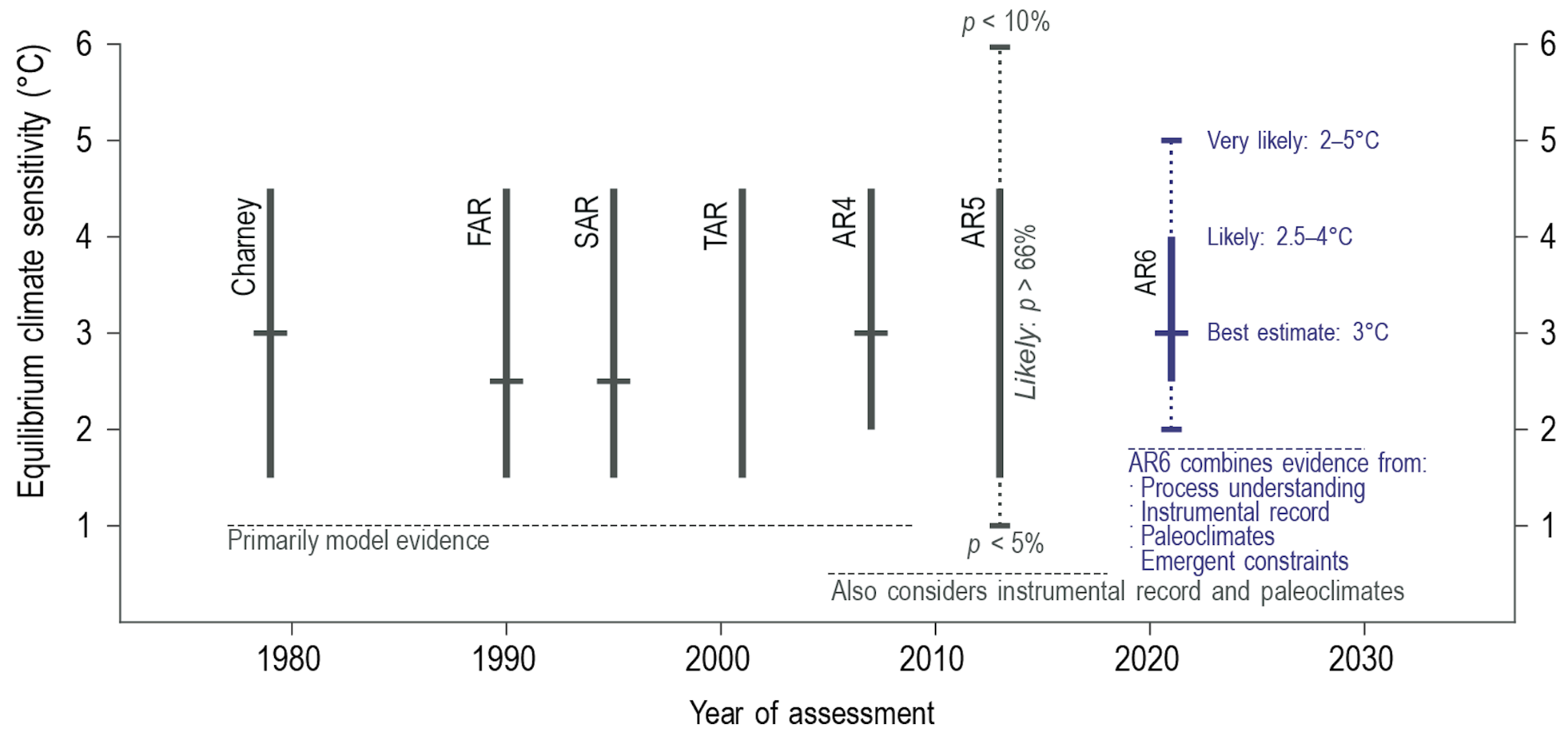
The magnitude of global surface-air temperature change associated with future emissions and thus atmospheric concentrations of the main drivers (well mixed greenhouse gasses and aerosols) is associated with the system’s sensitivity to these changes. Uncertainties about this central quantity still exist, but the range that is to a large part driven by aerosols and how they interact with clouds, has been further reduced in the recent years since Charney et al. (1979) by using observational constraints (Sherwood et al. 2020; Hausfather et al. 2020; Brunner et al. 2020; Gillett et al. 2021; Ribes et al. 2021). The figure below shows the evolution of best estimates of climate sensitivity over the years.

Figure: Evolution of the equilibrium climate sensitivity of the global surface air temperature. First, Second, and Third Assessment Report: FAR, SAR, and TAR; Assessment Reports 4, 5, and 6: AR4, AR5, AR6. From Charney et al. (1979) to AR6 (Source: IPCC, 2021).

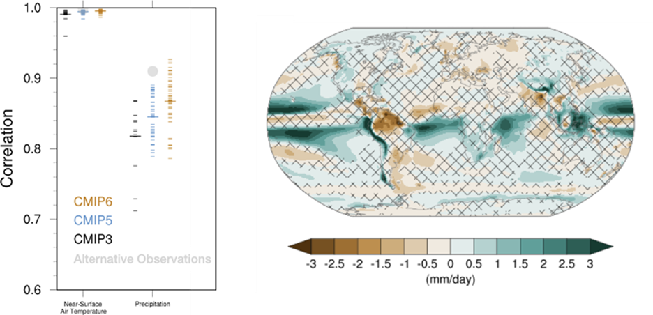
The spatial skill of models in reproducing the observed patterns continues to improve, with temperature historically already well represented, and precipitation gradually improving.

The panels show the progression of the spatial correlation of temperature and precipitation of CMIP models against reference observations (left panel) and a global map of precipitation bias of the CMIP6 multi-model ensemble mean (right panel). Temperature structures have historically been very well represented (indicated by very high correlation coefficients), while precipitation patterns have improved more gradually. However, precipitation “skill” also suffers from the fact that there are large differences between observational datasets, and thus assessing the actual quality is more challenging. Still, the continuous increase in correlation against observations is obvious. The right panel shows the spatial structure of the biases, where the tropical regions stand out for their large biases – part of which can be related to the coarse spatial representation in climate models (i.e. coastal upwelling areas are not well resolved), but also the systematic errors due to double Intertropical Convergence Zone (ITCZ) representation and tropical convection dynamics [5].

Figure: Improvements of temperature and precipitation pattern correlation over the course of three CMIP generations (left panel). CMIP6 multi-model precipitation bias (right panel), with crossed lines indicating regions with conflicting signal. Source: ESMVal Tools, Eyering et al., 2020.

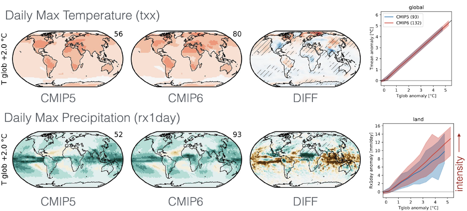
Some of the differences in climate modeling results have decreased over time; others have increased.

In the figure below, differences between CMIP5 and CMIP6 results are very small in the global temperature field, except in the Arctic where CMIP6 shows somewhat larger changes in sea ice. For precipitation, however, more differences are seen in the tropics with often increased intensity of daily maximum precipitation compared to the earlier generation of models. This reflects the development process in the different modeling groups that are aiming toimprove the utility of the model output, where extreme precipitation is a climate variable that is in high demand (e.g., Trenberth et al. 2003; Seneviratne et al. 2012).

Figure: Comparison of changes in daily maximum temperature (top) and daily maximum precipitation (bottom) between CMIP5 and CMIP6. The right panels show a summary of these changes relative to the global mean temperature. Temperature changes are well aligned between the two generations of CMIP, but precipitation projections show a distinct increase in intensity in the new CMIP6 models (red) compared to earlier versions of CMIP5 (blue). Source: IPCC, 2021.

Climate models have also improved in representing climate variability across a broad range of timescales.

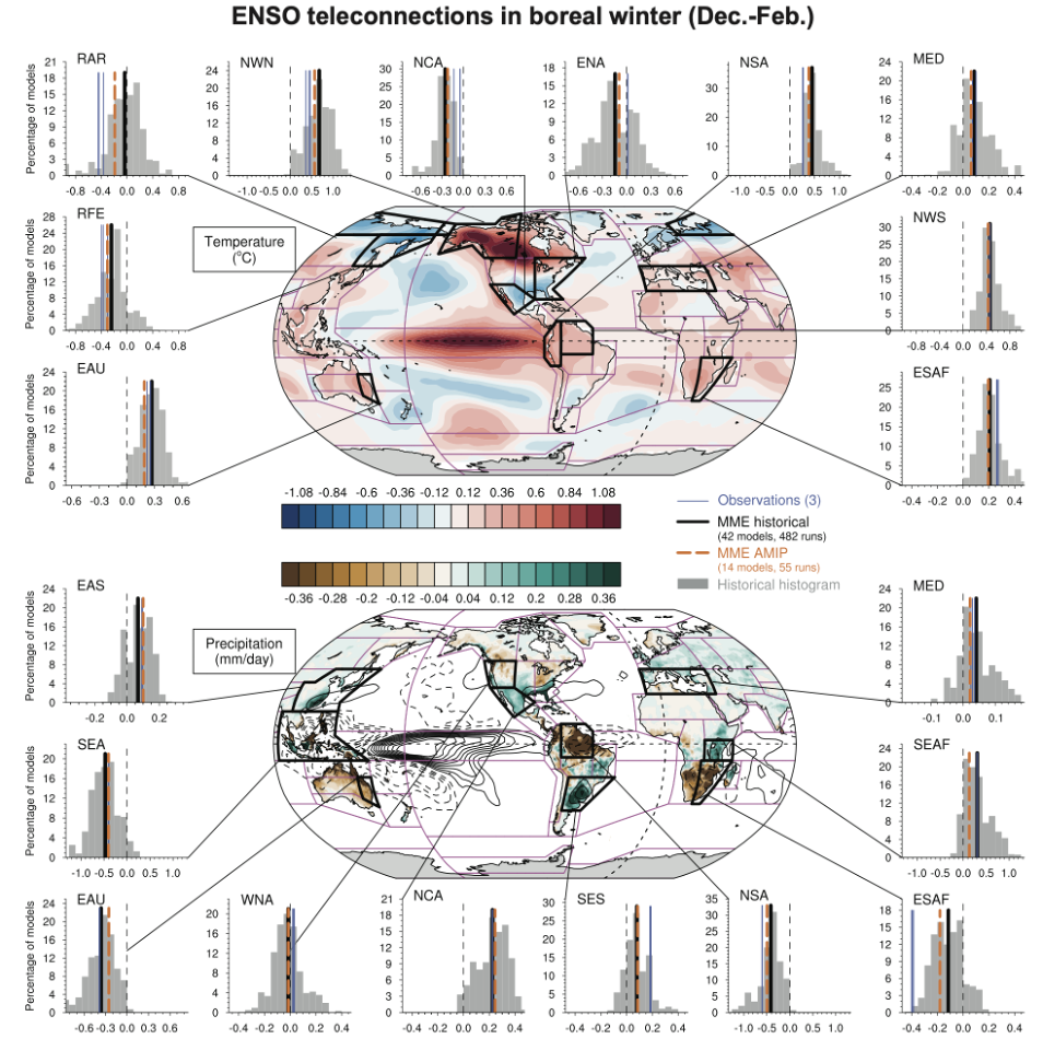
Diagnostics comparing the global models against observations demonstrate continued improvements (Lauer et al. 2020). The figure below illustrates the spatial structure of El Niño – Southern Oscillation (ENSO) related variability and how models manage to reproduce the key features. Overall reasonable direction and magnitudes of anomalies can be seen, though challenges in duration and frequency (power spectrum) of events remain. However, it also needs to be kept in mind that for many of the impacts related to potential changes in the statistics of these modes of variability, the observational record is often too short to allow for a robust identification of trends on the mode as well as the stability of teleconnections (see e.g., Krokos et al., 2019). While we can describe what global models project in terms of trends of these modes, a validation of these trends through theory and observations is often missing.

Figure: El Nino-Southern Oscillation teleconnections in boreal winter as represented in CMIP6. (Source: IPCC, 2021)

In conclusion, climate modeling has made steady improvements over the years and now represents a strong basis to inform adaptation and mitigation action.

The GCM models of the Earth system have been able to provide decision makers with a growing confidence in the way processes that dominate future climate under different scenarios are reflected in modeling frameworks. The above examples illustrate the increasing accuracy by which temperature, precipitation and other large-scale patterns are effectively reproduced within models under different socioeconomic development scenarios. In fact, models are now so detailed, that they can be used to spot errors in the observational record (e.g., Santer et al. 2003; 2011), even as the observational record has been used to validate climate models.

4.5 Earth system climate modeling – ongoing challenges

Despite the progress, uncertainties remain regarding climate models’ ability to represent the earth-climate system.

Importantly, reducing these uncertainties will not change the fundamental, robust conclusion that climate change is largely driven by anthropogenic emissions of GHGs. However, improving the predictive capability of climate models at the spatial and temporal scales necessary for decision-making will help reduce criticism when discussing the uncertainties of climate modeling results. There are several scientific challenges that the climate modeling community continue to work on, with the following bullets a sample of such challenges.

Aerosol-cloud interactions

One of the largest modeling challenges is associated with the processes of aerosol-cloud interactions (Gettelman and Sherwood, 2016). Even when the composition of aerosols are generally known - and thus one can calculate their “direct radiative effect” (e.g. Osipov et al. 2015) - how these particles interact with clouds and influence cloud structure and evolution, and then how they influence precipitation (the “indirect effect”, see Shine et al. 2015; Anisimov et al., 2018; Francis et al. 2021), is highly uncertain and can depend on numerous, very detailed processes. The large uncertainties in aerosol forcing are associated with these issues. The consequences of these processes, however, are important because they have a substantial influence on the sensitivity of the climate system (Sherwood et al. 2020). To make matters worse, potential future change in aerosol composition will continue to challenge the ability to accurately model aerosol-cloud interactions. Improved understanding of cloud-aerosol dynamics will remain a high priority for years to come.

Ice sheet dynamics.

A newer topic within CMIP is the simulation of the response of polar ice sheets to the changing climate. Earlier generations of models did not contain dynamic ice sheet components and thus were hampered in estimating future changes in global sea level. Several of this latest generation of models include polar ice sheets and thus the model-based estimates of sea level have been corrected upwards. However, the lack of long-term observations in the vicinity of the ice sheets on ice sheet stability and the ocean-ice interface limits the confidence in the results at the present time.

Carbon cycle feedback loops

Another focal point of development is centered on the carbon cycle feedback, and how it interacts with vegetation and land use (Friedlingstein et al. 2014). The carbon cycle contains many feedback mechanisms, some of which are positive and speed up warming trends (e.g., an increase of dead trees in a forest reduces gross primary productivity which means less carbon dioxide is being absorbed from the air for photosynthesis) and some of which are negative and serve to slow the warming trend (e.g., ocean buffering resists changes in ocean pH to some extent). Some feedbacks are highly local and extremely sensitive to environmental conditions. Therefore, even the sign over large areas are difficult to constrain. This topic too will remain as a priority challenge in future CMIP efforts.

Artificial intelligence

As mentioned above, the role of ML/AI approaches within models and in the post-processing of outcomes will dramatically change in the years ahead. The opportunities that these computationally efficient techniques offer is difficult to exaggerate. Still, there will be the problems of stationarity, and physics-based non-linear dynamics that will have to be overcome. Nevertheless, a new class of tools is likely to emerge that will increasingly influence how we approach simulations and explore ranges of impacts. The activities towards “Digital Twins” of the Earth will heavily rely on these methods.

Ground truthing

Finally, the challenge of maintaining continued, high-quality observational networks remains a serious challenge in many parts of the globe despite the increase in capabilities of using remotely sensed information from ever more capable satellite platforms. Still, without ground truthing, there will continue to be challenges in estimating critical parameters such as precipitation (Song and Bai, 2016, Chen et al. 2019).

For more information on the history of GCM’s and future climate datasets, please visit Learn More

Ch4 References

Abramowitz, G. et al., 2019: ESD Reviews: Model dependence in multi-model climate ensembles: weighting, sub-selection and out-of-sample testing. Earth System Dynamics, 10(1), 91–105, doi:10.5194/esd-10-91-2019.

Anisimov, A. et al. 2018: Observations and cloud-resolving modeling of haboob dust storms over the Arabian peninsula. Journal of Geophysical Research: Atmospheres, 123, 12,147–12,179. https://doi.org/10.1029/ 2018JD028486

Birkel, S.D., P.A. Mayewski, K.A. Maasch, A. Kurbatov, and B. Lyon, 2018: Evidence for a volcanic underpinning of the Atlantic multidecadal oscillation. npj Climate and Atmospheric Science, 1(1), 24, doi:10.1038/ s41612-018-0036-6.

Brunner, L. et al., 2020: Reduced global warming from CMIP6 projections when weighting models by performance and independence. Earth System Dynamics, 11(4), 995–1012, doi:10.5194/esd-11-995-2020.

Charney, J.G. et al., 1979: Carbon Dioxide and Climate: A Scientific Assessment. National Research Council (NRC). The National Academies Press, Washington, DC, USA, 34 pp., doi:10.17226/12181.

Chen, S. et al., 2019: Added Value of a Dynamical Downscaling Approach for Simulating Precipitation and Temperature Over Tianshan Mountains Area, Central Asia. Journal of Geophysical Research: Atmospheres, 124(21), 11051–11069, doi:10.1029/2019jd031016.

Deser, C., R. Knutti, S. Solomon, and A.S. Phillips, 2012: Communication of the role of natural variability in future North American climate. Nature Climate Change, 2(11), 775–779, doi:10.1038/nclimate1562.

Deser, C., A.S. Phillips, M.A. Alexander, and B. Smoliak, 2014: Projecting North American climate over the next 50 years: Uncertainty due to internal variability. Journal of Climate, 27(6), 2271–2296, doi:10.1175/jcli-d-13-00451.1.

Eyring, V. et al., 2016: Overview of the Coupled Model Intercomparison Project Phase 6 (CMIP6) experimental design and organization. Geoscientific Model Development, 9(5), 1937–1958, doi:10.5194/gmd-9-1937-2016.

Eyring, V. et al., 2020: Earth System Model Evaluation Tool (ESMValTool) v2.0 – an extended set of large-scale diagnostics for quasi-operational and comprehensive evaluation of Earth system models in CMIP. Geoscientific Model Development, 13(7), 3383–3438, doi:10.5194/gmd-13-3383-2020.

Fischer, E.M., U. Beyerle, and R. Knutti, 2013: Robust spatially aggregated projections of climate extremes. Nature Climate Change, 3, 1033–1038, doi:10.1038/nclimate2051.

Fischer, E.M., J. Sedláček, E. Hawkins, and R. Knutti, 2014: Models agree on forced response pattern of precipitation and temperature extremes. Geophysical Research Letters, 41(23), 8554–8562, doi:10.1002/2014gl062018.

Francis D., et al., 2021: Summertime dust storms over the Arabian Peninsula and impacts on radiation, circulation, cloud development and rain. Atm. Res., 250, doi:10.1016/ j.atmosres.2020.105364.

Friedlingstein, P. et al., 2014: Uncertainties in CMIP5 Climate Projections due to Carbon Cycle Feedbacks. Journal of Climate, 27(2), 511–526, doi:10.1175/jcli-d-12-00579.1.

Gettelman, A. and S.C. Sherwood, 2016: Processes Responsible for Cloud Feedback. Current Climate Change Reports, 2(4), 179–189, doi:10.1007/ s40641-016-0052-8.

Gillett, N.P. et al., 2016: The Detection and Attribution Model Intercomparison Project (DAMIP v1.0) contribution to CMIP6. Geoscientific Model Development, 9(10), 3685–3697, doi:10.5194/gmd-9-3685-2016.

Gillett, N.P. et al., 2021: Constraining human contributions to observed warming since the pre-industrial period. Nature Climate Change, 11(3), 207–212, doi:10.1038/s41558-020-00965-9.

Giorgi F. and W.J. Gutowski Jr., 2015: Regional Dynamical Downscaling and the CORDEX Initiative. Ann. Review of Environment and Resoruces, 40, 467-490, doi:10.1146/annurev-environ-102014-021217.

Gutowski Jr., W.J. et al., 2016: WCRP cOordinated Regional Downscaling eXperiment (CORDEX): a diagnostic MIP for CMIP6. Geoscientific Model Development, 9(11), 4087–4095, doi:10.5194/gmd-9-4087-2016.

Hausfather, Z., H.F. Drake, T. Abbott, and G.A. Schmidt, 2020: Evaluating the performance of past climate model projections. Geophysical Research Letters, 47, e2019GL085378, doi:10.1029/2019gl085378.

Hawkins, E. and R. Sutton, 2009: The Potential to Narrow Uncertainty in Regional Climate Predictions. Bulletin of the American Meteorological Society, 90(8), 1095–1108, doi:10.1175/2009bams2607.1.

Huntingford, C., E.S. Jeffers, M.B. Bonsall, H.M. Christensen, T. Lees, and H. Yang, 2019: Machine learning and artificial intelligence to aid climate change research and preparedness. Environmental Research Letters, 14, 124007, doi: 10.1088/1748-9326/ab4e55.

IPCC 2016: Paris Agreement: https://unfccc.int/sites/default/files/resource/parisagreement_publi-cation.pdf

IPCC, 2021: Climate Change 2021: The Physical Science Basis. Contribution of Working Group I to the Sixth Assessment Report of the Intergovernmental Panel on Climate Change [Masson-Delmotte, V., P. Zhai, A. Pirani, S.L. Connors, C. Péan, S. Berger, N. Caud, Y. Chen, L. Goldfarb, M.I. Gomis, M. Huang, K. Leitzell, E. Lonnoy, J.B.R. Matthews, T.K. Maycock, T. Waterfield, O. Yelekçi, R. Yu, and B. Zhou (eds.)]. Cambridge University Press, Cambridge, United Kingdom and New York, NY, USA, 2391 pp. doi:10.1017/9781009157896.

Khodri, M. et al., 2017: Tropical explosive volcanic eruptions can trigger El Niño by cooling tropical Africa. Nature Communications, 8(1), 778, doi:10.1038/s41467-017-00755-6.

Kirchmeier-Young, M.C., H.Wan, X. Zhang, and S.I. Seneviratne, 2019: Importance of Framing for Extreme Event Attribution: The Role of Spatial and Temporal Scales. Earth’s Future, 7(10), 1192–1204, doi:10.1029/2019ef001253.

Krokos G., et al., 2019: Natural climate oscillations may counteract Red Sea warming over the coming decades. Geophys. Res. Lett., 46, 3454-3461, doi:10.1029/2018GL081397.

Lauer, A. et al., 2020: Earth System Model Evaluation Tool (ESMValTool) v2.0 – diagnostics for emergent constraints and future projections from Earth system models in CMIP. Geoscientific Model Development, 13(9), 4205–4228, doi:10.5194/gmd-13-4205-2020.

Lehner, F. et al., 2020: Partitioning climate projection uncertainty with multiple large ensembles and CMIP5/6. Earth System Dynamics, 11(2), 491–508, doi:10.5194/esd-11-491-2020.

Maher, N., S. McGregor, M.H. England, and A. Gupta, 2015: Effects of volcanism on tropical variability. Geophysical Research Letters, 42(14), 6024–6033, doi:10.1002/2015gl064751.

Maher, N. et al., 2019: The Max Planck Institute Grand Ensemble: Enabling the Exploration of Climate System Variability. Journal of Advances in Modeling Earth Systems, 11(7), 2050–2069, doi:10.1029/2019ms001639.

Maher, N., S.B. Power, and J. Marotzke, 2021: More accurate quantification of model-to-model agreement in externally forced climatic responses over the coming century. Nature Communications, 12(1), 788, doi:10.1038/s41467- 020-20635-w.

Marotzke, J. and P.M. Forster, 2015: Forcing, feedback and internal variability in global temperature trends. Nature, 517(7536), 565–570, doi:10.1038/ nature14117.

Masson, D. and R. Knutti, 2011: Climate model genealogy. Geophysical Research Letters, 38(8), L08703, doi:10.1029/2011gl046864.

Moss, R.H. et al., 2010: The next generation of scenarios for climate change research and assessment. Nature, 463, 747, doi:10.1038/nature08823.

Murphy, J.M. et al., 2004: Quantification of modelling uncertainties in a large ensemble of climate change simulations. Nature, 430(7001), 768–772, doi:10.1038/nature02771.

Nakicenovic N., and R. Swart, 2000: Special report on emissions scenarios (SRES). Cambridge University Press, Cambridge, UK.

O’Gorman, P.A., and J. G. Dwyer. 2018: Using machine learning to parameterize moist convection: Potential for modeling of climate, climate change, and extreme events. Journal of Advances in Modeling Earth Systems, 10, 2548-2563, doi:10.1029/2018MS001351.

O’Neill, B.C. et al., 2016: The Scenario Model Intercomparison Project (ScenarioMIP) for CMIP6. Geoscientific Model Development, 9(9), 3461– 3482, doi:10.5194/gmd-9-3461-2016.

Osipov S, et al. 2015: Diurnal cycle of the dust instantaneous direct radiative forcing over the Arabian Peninsula. Atmos. Chem. Phys, 15, 9537-9553, doi:10.5194/acp-15-9537-2015.

Otterå, O.H., M. Bentsen, H. Drange, and L. Suo, 2010: External forcing as a metronome for Atlantic multidecadal variability. Nature Geoscience, 3(10), 688–694, doi:10.1038/ngeo955.

Riahi K, et al., 2017: The Shared Socioeconomic Pathways and their energy, land use, and greenhouse gas emissions implications: An overview. Glob. Env. Change, 42, 153-168, doi:10.1016/j.gloenvcha.2016.05.009.

Ribes, A., S. Qasmi, and N.P. Gillett, 2021: Making climate projections conditional on historical observations. Science Advances, 7(4), 1–10, doi:10.1126/sciadv.abc0671.

Rogelj, J. et al., 2018: Mitigation Pathways Compatible with 1.5°C in the Context of Sustainable Development. In: Global Warming of 1.5°C. An IPCC Special Report on the impacts of global warming of 1.5°C above pre- industrial levels and related global greenhouse gas emission pathways, in the context of strengthening the global response to the threat of climate change, [Masson-Delmotte, V. et al. (eds.)]. In Press, pp. 93–174, www.ipcc.ch/sr15/ chapter/chapter-2.

Rowell, D.P., 2012: Sources of uncertainty in future changes in local precipitation. Climate Dynamics, 39(7–8), 1929–1950, doi:10.1007/s00382-011-1210-2.

Saffioti, C., E.M. Fischer, and R. Knutti, 2017: Improved Consistency of Climate Projections over Europe after Accounting for Atmospheric Circulation Variability. Journal of Climate, 30(18), 7271–7291, doi:10.1175/jcli-d-16-0695.1.

Santer et al. 2003: Influence of satellite data uncertainties on the detection of externally forced climate change. Science, 300, 1280-1284.

Santer et al. 2011: The reproducibility of observational estimates of surface and atmospheric temperature change. Science, 334 ,1232-1233, doi:10.1126/science.1216273.

Seneviratne, S.I. et al., 2012: Changes in Climate Extremes and their Impacts on the Natural Physical Environment. In: Managing the Risks of Extreme Events and Disasters to Advance Climate Change Adaptation. A Special Report of Working Groups I and II of the Intergovernmental Panel on Climate Change [Field, C.B. et al. (eds.)]. Cambridge University Press, Cambridge, United Kingdom and New York, NY, USA, pp. 109–230, doi:10.1017/cbo9781139177245.006.

Sherwood, S.C. et al., 2020: An Assessment of Earth’s Climate Sensitivity Using Multiple Lines of Evidence. Reviews of Geophysics, 58(4), e2019RG000678, doi:10.1029/2019rg000678.

Shine, K.P., R.P. Allan, W.J. Collins, and J.S. Fuglestvedt, 2015: Metrics for linking emissions of gases and aerosols to global precipitation changes. Earth System Dynamics, 6(2), 525–540, doi:10.5194/esd-6-525-2015.

Smith, D.M. et al., 2016: Role of volcanic and anthropogenic aerosols in the recent global surface warming slowdown. Nature Climate Change, 6(10), 936–940, doi:10.1038/nclimate3058.

Song, S. and J. Bai, 2016: Increasing Winter Precipitation over Arid Central Asia under Global Warming. Atmosphere, 7(10), 139, doi:10.3390/atmos 7100139.

Taylor, K.E., R.J. Stouffer, and G.A. Meehl, 2012: An Overview of CMIP5 and the Experiment Design. Bulletin of the American Meteorological Society, 93(4), 485–498, doi:10.1175/bams-d-11-00094.1.

Towler, E., and Yates, D. 2021: Incorporating multiyear temperature predictions for water resources planning. Journal of Applied Meteorology and Climatology, 60(2), 171-183.

Trenberth K.E., A. Dai, R.M. Rasmussen, and D.B. Parsons, 2003: The changing character of precipitation. Bull. Am. Meteorol. Soc., 84(9), 1205-1218.

van Vuuren, D.P. et al., 2011: The representative concentration pathways: an overview. Climatic Change, 109(1–2), 5–31, doi:10.1007/ s10584-011-0148-z.

van Vuuren, D.P. et al., 2014: A new scenario framework for Climate Change Research: scenario matrix architecture. Climatic Change, 122(3), 373–386, doi:10.1007/s10584-013-0906-1.

Watson-Parris, D. 2021: Machine learning for weather and climate are worlds apart. Phil. Trans. Roy. Met. Soc., A, 379(2194): 20200098, doi:10.1098/rsta.2020.0098.

Wilby, R.L. and S. Dessai, 2010: Robust adaptation to climate change. Weather, 65(7), 180–185, doi:10.1002/wea.543.

Wilcox, L.J. et al., 2020: Accelerated increases in global and Asian summer monsoon precipitation from future aerosol reductions. Atmospheric Chemistry and Physics, 20(20), 11955–11977, doi:10.5194/acp-20-11955-2020.

Zanchettin, D., 2017: Aerosol and Solar Irradiance Effects on Decadal Climate Variability and Predictability. Current Climate Change Reports, 3(2), 150– 162, doi:10.1007/s40641-017-0065-y.

Zuo, M., W. Man, T. Zhou, and Z. Guo, 2018: Different Impacts of Northern, Tropical, and Southern Volcanic Eruptions on the Tropical Pacific SST in the Last Millennium. Journal of Climate, 31(17), 6729–6744, doi:10.1175/ jcli-d-17-0571.1

[1]

Radiative forcing is a measure of how the energy balance of the Earth–atmosphere system is influenced. The word ‘radiative forcing’ is used because these factors change the balance between incoming solar radiation and outgoing IR radiation within the Earth’s atmosphere.

[2]

Refers to the practice of modifying the fluxes (of heat and water) between the atmosphere and ocean in coupled atmosphere–ocean models. This modification is designed to minimize the climate drift that occurs during model integration. These flux adjustments are typically a function of location and season.

[3]

Refers to the mean of the impact variances for each climate model. The power spectrum of internal variability quantifies how variance is distributed over frequencies and is useful for identifying periodic behavior in time series.

[4]

The detailed summaries across the chapters of the Working group I report of the 6th Assessment Report of the IPCC provide an in-depth description of the state of knowledge within each of the components of the Earth’s climate system.

[5]

The double- ITCZ problem refers to the excessive precipitation that is produced in the Southern Hemisphere tropics, which resembles a Southern Hemisphere counterpart to the strong Northern Hemisphere ITCZ. It is arguably the most significant and most persistent bias of the global climate models.