Learn More…

Introduction to Climate Models

Introduction

Weather forecasters depend on numerical weather prediction (NWP) models to produce timely, accurate forecasts. We depend on these forecasts to make all manner of decisions from recreation choice to emergency response. As a community, weather forecasters understand the strengths and weaknesses of NWP models better than just about any other group. Every forecaster knows, for example, that model skill drops sharply with time and that NWP models struggle to produce accurate and precise forecasts more than a week into the future.

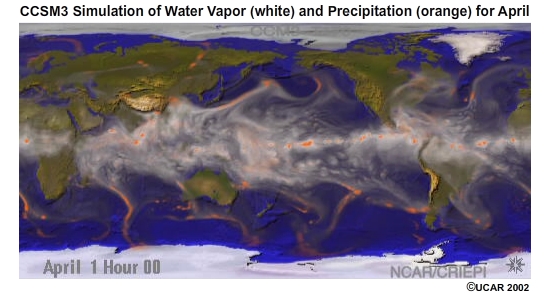
Climate models share a common heritage with NWP models. For example, this animation shows water vapor and precipitation for a period of several days. We see the same weather patterns produced by NWP models and observed in satellite images. In a climate simulation, the model would run for decades or centuries, rather than days. As a result, forecasters frequently wonder how a climate model can produce an accurate projection decades or centuries in the future, when NWP models cannot produce an accurate forecast at 10 days. The answer lies in the questions the respective models seek to address.

This module explains how climate models work. We explain not only how, but why climate models differ from weather models.

We have attempted to restrict the scope of this module to climate models, rather than climate science. We do however, draw upon climate science to illuminate the questions that climate models answer and to illustrate concepts with data from models and observations. For example, we do not attempt to explain the mechanics of El Nino-Southern Oscillation (ENSO), but we show examples of observations and model simulations of ENSO phenomena.

Why Model the Earth System?

Why do we model the climate system?

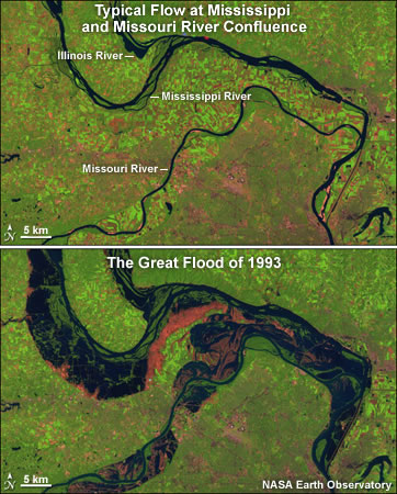
Since the start of the Industrial Revolution, greenhouse gases, principally carbon dioxide, have increased substantially in the atmosphere. The past several decades have seen a significant rise in global surface temperatures. The climate change associated with this warming may have profound impacts for society. For example, the frequency of extreme events, like the flooding that struck the midwest in 1993, may increase with a high toll on society.

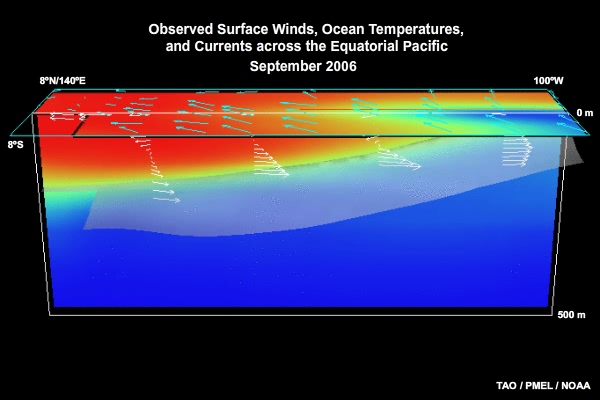
Understanding how climate changes in response to changes in the composition of the atmosphere and other factors drives climate research. Climate models provide a tool to understand how processes work and interact with each other. For example, El Nino/Southern Oscillation (ENSO) is a mode of climate variability that strongly influences weather in North America and beyond. It results from a complex interaction of atmosphere and ocean. This animation shows observed winds, ocean temperatures, and currents across the Equatorial Pacific through five years of an ENSO cycle. Successfully modeling the complex interactions that result in ENSO allows researchers to understand the roles of the processes involved and how they interact.

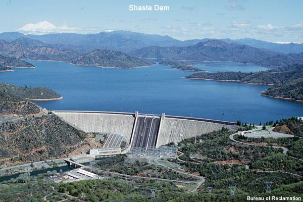
We also use models as a tool to look into the future, just as we use weather forecast models to make predictions. Both weather and climate models provide information for societal needs. For example, planning for future water and hydrologic needs requires looking far into the future. Building a dam, like the Shasta Dam shown here, requires a long lead time.

Global Energy Flows

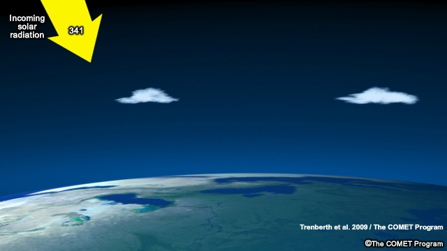
Solar energy drives the Earth’s climate system. Based on measurements from satellites and other instruments, we can trace the flow of energy through the climate system. Note that the numbers are best estimates in Watts per square meter as of 2009. We can expect these numbers to change as our observations and understanding improve.

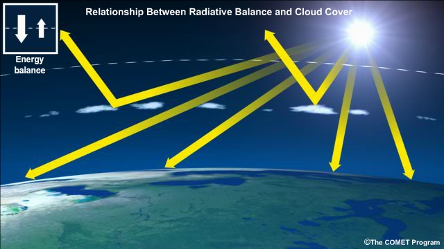
Energy comes into the climate system as shortwave solar radiation. Some of that energy reflects off clouds and the atmosphere back to space. Some more is absorbed by the atmosphere.

The rest makes its way to the surface, where most is absorbed but some is also reflected. The difference between the incoming and the reflected energy is the total available to the Earth’s climate system. About two-thirds of that is absorbed by the surface, while the rest is absorbed by the atmosphere.

Solar energy absorbed at the surface warms the surface, which radiates thermal, or longwave, radiation.

Some of that radiation makes it directly out to space through the so-called atmospheric window and some more is absorbed by clouds. There are also greenhouse gases in the atmosphere, particularly water vapor and carbon dioxide, that very efficiently absorb longwave radiation and radiate it.

Greenhouse gases radiate in all directions so that some radiated energy is directed upward toward space, with the remainder directed downward toward the surface.

Radiative transfer isn’t the only way that energy moves between the surface and the atmosphere. The surface also loses energy through evapotranspiration from plants and wet surfaces (latent heat), and through conduction (sensible heat).

Climate models need to account for all the processes that modulate this flow of energy. For example, clouds reflect, absorb, and radiate energy. Therefore, the cloud processes need to be accurately simulated in climate models. Similarly, vegetation strongly modulates energy flow by affecting albedo and evapotranspiration.

Earth’s Atmospheric Dynamics

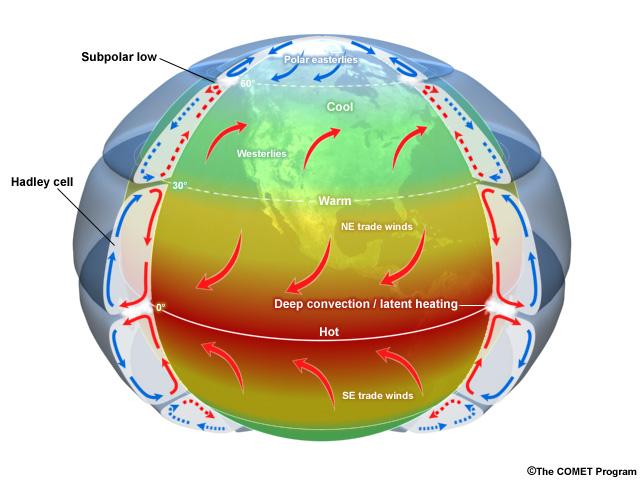
Incoming solar radiation is much stronger near the equator than near the poles. Atmospheric circulations develop in response to this unequal distribution. These circulations attempt to equalize this distribution by moving heat from warmer to colder regions. Climate models have to account for these large-scale circulations, such as Hadley cells, and the convective heating shown in this figure.

Storm Systems

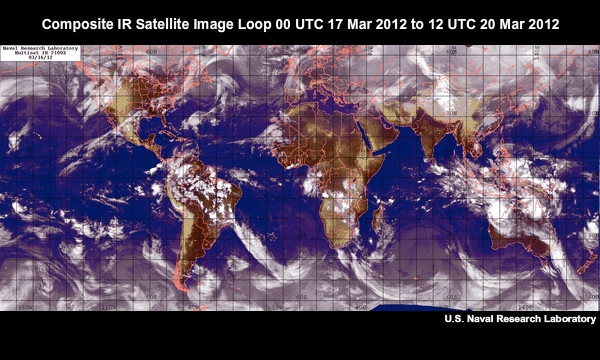
Furthermore, embedded within these planetary scale circulations are smaller-scale features that we call storm systems. They transport significant amounts of heat and energy around the planet. This loop of composite infrared satellite images shows storm systems pinwheeling across the globe at high latitudes. Note how the storms draw warm, moist, tropical air toward the poles.

Top of page

Earth’s Heat Transport

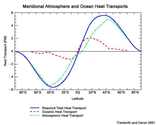
The result of long-term climatological circulation and short-term storm systems is the net transport of heat from low latitudes to high latitudes. This figure, based on observations, shows the total amount of energy (in petawatts or quadrillions of watts) that’s transported toward both poles by the atmosphere, shown in green, and by the ocean, shown in red. While the atmosphere transports most of the heat out of the tropics and toward the poles, the ocean also plays a significant role. Thus climate models need to simulate oceanic processes in addition to atmospheric ones.

Predictability of Weather and Climate

Weather versus Climate

The key difference between weather and climate is really a matter of time scale.

Weather is what we experience over the course of hours, days, and weeks.
Climate is the average of weather over years, decades, and longer.

Or, as the old adage goes: climate is what you expect, weather is what you get.

Forecast models are used to predict specific weather events. To do that, they start with the initial conditions and simulate how those conditions will evolve with time. Getting the initial conditions right turns out to be very important in forecasting weather events. The goal of those who develop and use these weather forecast models is to predict weather with enough accuracy to help those who may be affected by it.

On the other hand, climate models are used to generate the statistics (such as the mean and variability) of weather phenomena, not predict the time and place at which the phenomena will occur. So, while climate models simulate weather phenomena, they are not dependent on initial atmospheric conditions to the extent that weather forecast models are. Initial ocean conditions can affect the simulated climate over the course of several years (eg. El Nino/La Nina) to a decade or more.

Initial Condition vs Boundary Condition

-

In modeling terms, the difference between weather and climate is what we call an initial condition problem versus a boundary condition problem. Initial conditions are the starting point, the initial state of variables like wind, temperatures, pressure, and moisture. Boundary conditions, in contrast, are values prescribed by the modeler. Examples include the intensity of solar radiation and composition of the atmosphere. Weather depends on initial conditions, while climate on decadal and longer time scales depends primarily on boundary conditions.

Imagine we are looking at two forecast model runs starting from the same initial value, representative of the spring or fall season in either the Northern or Southern Hemisphere: Let’s force one set of forecasts with summer incoming solar radiation. The result is a prediction of temperature that oscillates up and down and gradually warms.

Now take that model and run it several more times with summer solar forcing, starting each run with slightly different initial conditions, just like weather forecasters do with model ensembles. The forecasts diverge with time, but stay within some gradually warming forecast envelope. The details of the forecast, just like weather, depend critically upon the initial conditions of the model run.

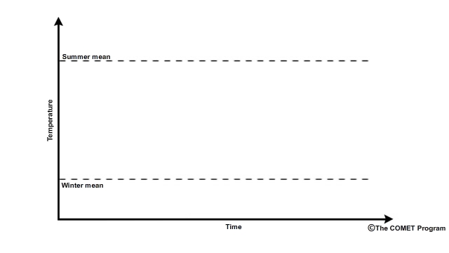
Next, repeat the process, but use winter solar forcing. It quickly becomes clear that the summer state is significantly warmer than the winter state.

The variance within the summer and winter ensembles results from slight changes in the initial conditions.

The difference between the summer and winter forecasts, or seasonality, results from a difference in boundary conditions.

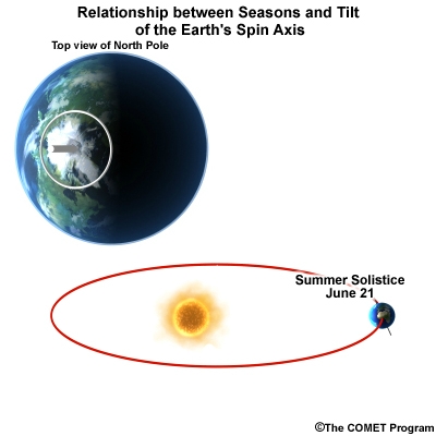
If this were a location in the U.S., we know that it will be warmer in the summer, on average, than in the winter. The boundary condition that differs from summer to winter is the intensity and daily amount of incoming solar radiation reaching the Earth’s surface, which is directly related to the tilt of the Earth with respect to the sun. Seasonality is a boundary condition. The Northern Hemisphere gets more sunlight in summer than in winter.

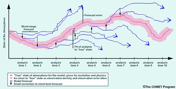
On the other hand, the drift and spread between different forecasts within the summer and winter ensembles reflects a difference in initial conditions. This graphic illustrates how model forecasts continually drift away from the true state of the atmosphere. As a result, forecasters frequently re-initialize weather models to better match current observations, typically several times per day.

For climate models, it’s the boundary conditions that matter. Initialization does not affect the long-term statistics that the models are designed to generate for periods of decades to centuries.

Prediction vs Projection

Another way to look at weather versus climate is looking at it as a forecast challenge.

Weather forecasters have a strong grasp of the fundamental mechanics of their task. If you know the initial conditions, you can predict how the weather is going to evolve for some time going forward. This is why so much effort is expended obtaining and assimilating observations for numerical weather prediction. And by extension, a crucial step in the forecast process is to evaluate the model initialization by comparing the model analysis against current observations.

Making an ENSO forecast or a seasonal outlook of precipitation is structurally no different than making a daily weather forecast. Why? Because they both assume you have a good understanding of how the basic system works. And because you know how it works, if you know the initial conditions, you can predict how it’s going to vary going forward for some time into the future. Whether that’s a 24-hr forecast or a seasonal outlook, it’s structurally the same. The objective of such a forecast is the same, too: to produce a prediction for a given location for a given time period.

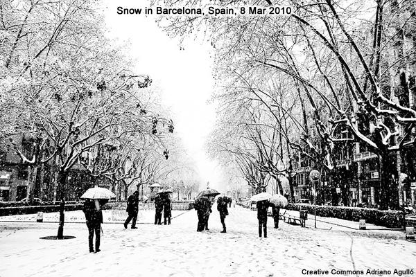
But there’s a limit to predictability. You’ve undoubtedly heard of Lorenz’s Butterfly: the allegory of how the flap of the butterfly’s wings over Brazil leads to a thunderstorm a week later. Small differences in the initial conditions, things we can’t even measure, will grow and contaminate the solution for a forecast. As a result, forecasters can’t predict if there will be snow on New Year’s day or rain on the summer solstice next year. That’s not because the weather model is no good, or we don’t understand the physics well enough. It’s due to the chaotic nature of the system.

When it comes to longer-term climate problems, those determined over decades to centuries, it’s a different challenge. We’re not interested whether in the year 2083 we’re going to have El Nino or La Nina, so the initial conditions don’t concern us. We’re interested in how the statistics of the climate system will change in response to changing boundary conditions.

Using our knowledge of how the climate system works, we want to know how factors that change the flow of energy will change the climate statistics. If the sun gets brighter, incoming energy increases. If the amount of carbon dioxide in the atmosphere increases, it changes how the atmosphere absorbs infrared radiation and, hence, changes the flow of energy through the system. If forest, which is dark, is replaced by crops and pastures that are brighter, the surface albedo changes. These are all examples of changes in boundary conditions. The physics are the same as those in weather prediction, but we’re solving a different problem.

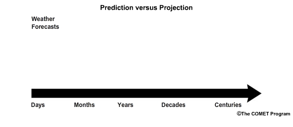
To distinguish between the questions addressed by weather and climate models, scientists use different terms. Projection refers to how the statistics of the climate system will change in response to changing boundary conditions. Prediction refers to the short-term evolution of the climate system from an initial state under constant boundary conditions.

Boundary Conditions

Boundary conditions in climate models all affect the way that energy is absorbed or exchanged in the climate system. Boundary conditions are not predicted by the model and must be specified. Some boundary conditions are natural, and others are influenced by human activities.

What are the boundary conditions in climate models?

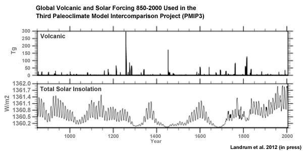
Natural boundary conditions include solar radiation and volcanic aerosols. Total solar insolation, observed at the top of the atmosphere, has varied by about 2 W/m2 around an average of about 1361 W/m2 over the past 1150 years. Large volcanic eruptions episodically inject large quantities of aerosols into the atmosphere, which reflects incoming solar radiation.

Natural forcing: How do we know?

Records of volcanic activity used to model past climate come from ice cores in the Arctic and Antarctic. For example, Gao et al. (2008) developed an index based on volcanic deposits in 54 ice core records. Based on the spatial distribution of the deposits and knowledge of stratospheric transport, they produced a volcanic forcing dataset as a function of month, latitude, and altitude for the past 1500 years.

The primary source of information on solar activity (before direct measurements were made) comes from concentrations of carbon-14, which is formed in the atmosphere by the collision of nitrogen-14 and cosmic rays from the sun. The carbon-14 is incorporated into plant material, where it slowly decays back to nitrogen-14. By measuring the carbon-14 concentration in trees that are well dated through their tree rings, and then accounting for the radioactive decay of carbon-14, we can determine the past concentration of carbon-14 in the atmosphere. From this, we can deduce the solar irradiance over time.

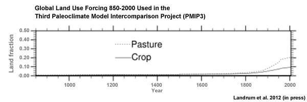
Human-influenced boundary conditions include changes at the surface and changes in the atmosphere. At the surface, cutting forest for pasture and crops changes surface reflectivity and moisture, heat, and momentum exchanges between land and atmosphere.

Land use: How do we know?

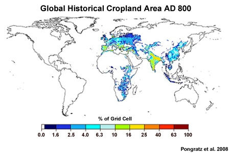
Land use reconstructions for times prior to the 20th century are based on population estimates and historical relationships of land use for different population densities. The calculations are done country-by-country to account for regional differences like crop types, farming technology, and diet. All the reconstruction methods largely rely on the similar historical population estimates. The results are gridded maps of land use through time.

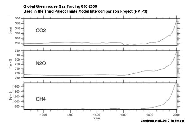
In the atmosphere, the most important changes are those that affect greenhouse gases. Greenhouse gases, principally water vapor and carbon dioxide, keep Earth habitable by absorbing enough long-wave radiation to keep surface temperatures tens of degrees Celsius warmer than they would be otherwise. These graphs show a rapid rise in different greenhouse gases over the past 2 centuries, primarily due to burning of fossil fuels.

Human emissions of atmospheric aerosols also alter the Earth’s energy balance. Depending on the composition of the aerosols and where they are, they contribute to both warming and cooling of the climate. Overall, aerosols are thought to contribute a cooling effect equal to about half of the warming caused by greenhouse gases when averaged over the globe.

Greenhouse gases: How do we know?

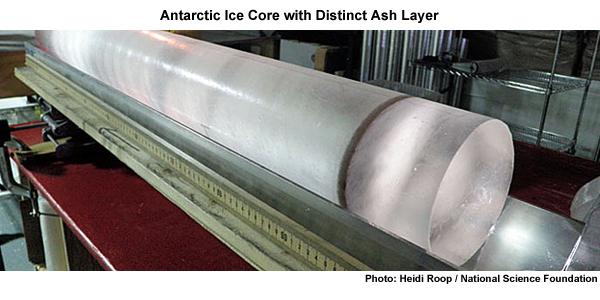
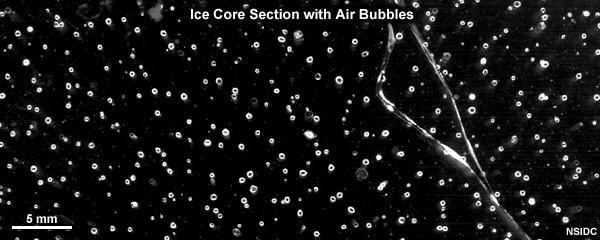
The concentration of greenhouse gases for climate reconstructions is based on measurements of the composition of air bubbles preserved in glacial ice in Antarctica. This photograph shows air bubbles trapped from an ice core from Antarctica. The prolonged darkness in winter and prolonged sunlight in summer leads to easily recognized and counted annual layers in the ice, yielding a high-resolution record of changes in atmospheric composition.

Building a Climate System Model

Physical Basis of Weather and Climate Models

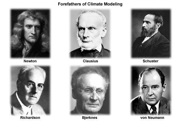
The modeling of both weather and climate share a deep history and common pedigree based on fundamental laws of physics whose discovery goes back, in some cases, hundreds of years. The equations and calculation methods used in the models can be traced back to the work of giants in the field and direct applications of the fundamental laws of physics, such as

Sir Isaac Newton’s laws of motion,
Rudolf Clausius’ 1st law of thermodynamics, and
Arthur Schuster’s governing equations of radiative transfer.

These scientists deduced the basic laws of physics that are the basis of any good climate and weather model.

In the 20th century, scientists applied these fundamental laws to the atmosphere:

Vilhelm Bjerknes, who wrote the equations that we use to forecast the wind in weather and climate models,
Lewis Richardson, the father of numerical weather forecasting, and
John von Neumann, who led the first team of scientists that successfully ran a numerical forecast model on a computer.

From this lineage we can see how weather and climate models developed from a common heritage, rooted in fundamental physics. Some people, when they hear the word “model”, believe that the equations used to describe physical processes are loosely constrained and can be easily “tweaked” to get whatever answer the modeler wants. That is not the case.

Resolved Dynamical Processes

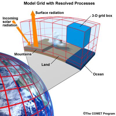
To directly simulate processes in Earth’s climate system, we need to create a set of equations using the fundamental laws of physics. These are called the equations of motion or primitive equations, and are used by both climate and NWP models. These equations balance forces acting in three dimensions, conserve mass, and track the temperature of each grid box. There are also equations that track the amount of moisture and other trace products that move in and out of grid boxes.

To solve these equations for Earth, we create a grid structure on which to make the calculations. This structure involves vertical columns of air sliced into horizontal layers over the full Earth for global models, or a portion of it for regional models. Finally, we solve the equations at the center point of each model grid box, at fixed, predetermined time intervals.

Early climate and weather models had grid cells that measured 300-400 km on a side. As of 2012, the NWP models have grid boxes as small as 1.5 km on a side or even a little less. Climate models are now run at a resolution as high as about 50 km.

Sub-grid Scale Processes and Parameterization

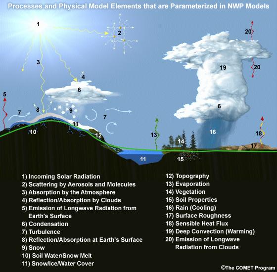
Even in high resolution models, some weather and climate processes are too small in scale to be calculated directly, and always will be, even though their impacts are important to weather and climate systems. These sub-grid scale processes, such as cumulus convection and radiative transfer of solar and longwave radiation, indirectly affect the climate and weather variables (the “resolved” variables) calculated on the grid. These indirect effects are determined by what is called “parameterization”.

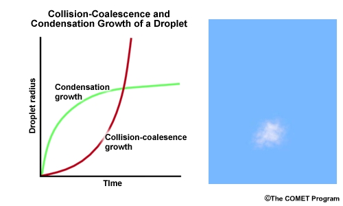
Parameterizations are designed using observations and the laws of physics; they are not a “best guess”. Take the example of a model representation of cloud microphysics. Conservation laws dictate the mass of water going in and out of a grid box. Vapor in the model condenses according to observationally based thresholds of relative humidity, forming “clouds”. Physical processes lead from clouds to the formation of droplets that then fall to grid boxes below as rain or snow, also based on observational evidence from within clouds.

Thus, the parameterization of clouds, although subject to many unknowns, is based on a combination of the conservation of mass and energy and an empirical understanding of cloud formation, grounded in observations. Using those properties, modelers create parameterizations for cloud processes that operate within model grid layers when appropriate environmental conditions are met.

Parameterizations do bring with them uncertainty. Some processes are better understood than others. But this is true of all model processes. Even the numerical representation of the laws of motion comes with uncertainty. There is no unique way to write the numerical solutions for resolved processes, like motion, and they all have some error associated with them. This is equally true for both weather models and climate models. Even so, uncertainty in weather and climate models is decreasing as our understanding of climate and weather processes further improves and computing power continues to increase.

Climate Model Evolution

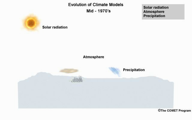
With the development of digital computers in the 1950s, it became theoretically possible to develop weather and climate models. Forecasting short-range weather with NWP models got attention first. Scientists only began to develop computerized climate models (also known as general circulation models or GCMs) in the late 1960s to early 1970s, but used the same equations as in NWP models.

Many details in early climate models (for example, sea surface temperatures and land/sea ice) had to be set to fixed or seasonal values because they could not be calculated: computational resources were insufficient and/or the processes involved were not well understood.

As our physical understanding of ocean, land, and ice processes advanced and computing power increased, scientists were able to add more climate processes and improve existing ones. For instance, models that realistically simulate overturning ocean circulation and its interaction with the atmosphere replaced prescribed ocean surfaces. Realistic land surface models replaced simple “bucket” models to better simulate vegetation effects on moisture, momentum, and heat transfer between the land and the atmosphere. The effect of aerosols, both natural and those generated by human activities, was also added. The inclusion of aerosols resulted in climate models capturing the temporary halt to increasing average global temperature during the mid-20th century, an effect that was not previously simulated.

More recently, scientists have added processes with long time scales or complicated physics and chemistry. These include the carbon cycle, atmospheric chemistry, and a biosphere capable of responding to model climate change (for example, vegetation cover changing from tundra to forest in response to predicted warming). Scientists have also added interactions between land and sea ice and the rest of the climate model.

Some of the processes included in climate models are relatively straightforward, while the impact of others needs to be more crudely estimated because of their characteristic time or space scales. In the next section, we will talk about how these processes are included in climate models.

Model components

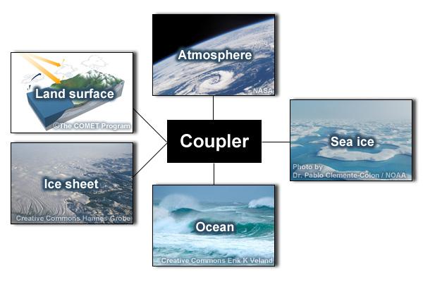
The components that go into a climate model include an atmosphere model, ocean model, land model (including snow and land ice), and sea ice model. A coupler manages the interactions between the different components, accommodating different grids, resolution, and time steps.

In contrast, NWP models mostly include just the atmosphere. The ocean, land, and ice are prescribed quantities with values derived from current satellite observations, climatology, or a mix of both. These values do not change much over the course of a weather forecast period, so they can be fixed.

Atmospheric Model

The atmospheric component of the climate model is very similar to a numerical weather prediction model. The model solves for both resolved processes, like motion, and parameterized processes, like cloud physics.

The model numerically solves the equations of motion at each grid point. In other words, the model directly simulates motion in the atmosphere between grid layers by balancing the pressure gradient force, Coriolis effect, and forces resulting from curvature in the flow.

There are also parameterized dynamics for aspects of atmospheric flow too small to resolve, such as gravity wave drag. We know from theory and observations that mountains generate gravity waves that propagate up into the atmosphere and transport momentum from the surface up into the atmosphere. This affects elements of the larger-scale flow such as the placement of the jet stream and storm tracks and the location and strength of planetary scale atmospheric waves.

Most physical processes must be parameterized. These include the following:

Radiative transfer, or how sunlight and long-wave radiation propagate up and down through the atmosphere.
Processes related to cloud formation resulting from both large-scale (resolved) lifting and from sub-grid scale convective processes. Traditionally, these processes have been hardest to parameterize.
Boundary layer and surface exchange processes that occur on scales much smaller than a typical grid box.
Dissipation of kinetic energy or momentum away from the boundary layer.

None of these processes are unique to climate models. Every weather forecast model includes them, too. If you look “under the hood” of any weather model, this is what you’re going to find.

Ocean Model

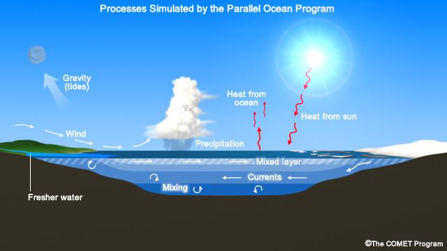
In order to adequately simulate climate, models must include the ocean. After all, most of the heat in the climate system is stored in the ocean. Furthermore, much of the natural variability in the climate system is controlled by oscillations in the ocean that are closely coupled to the atmosphere.

In contrast, NWP models use set ocean conditions, typically using satellite observations of sea surface temperatures, which are held constant through the course of a model run.

There are several important differences between the ocean and atmosphere that affect climate modeling:

Ocean processes operate over much longer time scales when compared to atmospheric processes. Complete mixing of the ocean takes centuries, and thus changes in forcing can take decades to appear in the ocean.
Ocean observations are sparse, which makes verification of model results more difficult. While satellites provide many observations of the surface, deep profiles come largely from drifting buoys that yield only about 300 profiles per day from the top 750 meters.

In many respects, ocean models are quite similar to atmospheric models; the equations of motion are largely the same. There are, however, some notable exceptions:

Ocean models are forced entirely at the surface
Ocean models need to account for salinity, which plays a large role in determining density
Surface currents are largely wind driven

Current climate models may now include an ocean ecosystem model. This model can be used as a component of the global carbon cycle model. It also enables a feedback from biogeochemistry to the ocean physics whereby the calculated chlorophyll content impacts the absorption of solar radiation in the ocean.

Land Model

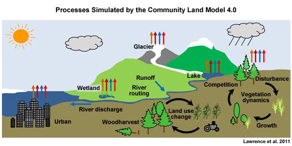
Climate models also need to account for what’s happening on land that influences climate. Land processes play an important role in exchanges of energy, moisture, and carbon with the atmosphere and ocean.

Land models have become far more sophisticated over the last 20 years. In the “old days,” just 20 or 30 years ago, models accounted for things like energy exchange between the atmosphere and land in very simple ways. Land model developers have replaced these simple schemes with more detailed simulations. Among other things, these simulations now account for

Energy and water exchange between different types of vegetation,
Vegetation effects on wind flow,
Interactive ecosystems that evolve with changing climate conditions,
A complete water cycle with infiltration, aquifers, groundwater, and surface flow,
Water, carbon, and nitrogen exchanges between soil, plants, and atmosphere, and
Freshwater runoff into the ocean, which affects salinity, which can then affect circulation.

Ice Models

Ice plays an important role in the climate system due to its high albedo. Ice-covered areas reflect a very high percentage of incoming shortwave radiation. Thus the presence or absence of ice tends to have an inordinately large effect on climate with large feedbacks in coupled systems.

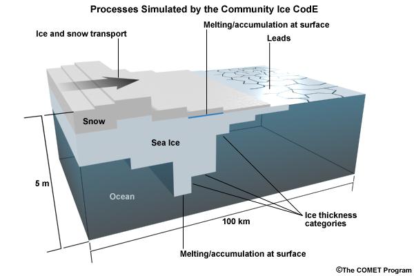
Sea ice forms from the freezing of seawater. Its presence or absence strongly impacts climate, both globally and locally. In addition to the albedo feedback described above, sea ice also acts as a barrier between the liquid ocean and the atmosphere and thus strongly alters the moisture flux, as well as latent and sensible heat fluxes. The formation of sea ice also plays a crucial role in the formation of the cold, saline water that drives deep ocean circulation.

In addition to the heat flux that results in freezing and melting, sea ice models simulate features including sea ice motion, formation of ridges and leads, melt ponds, and aerosol deposition.

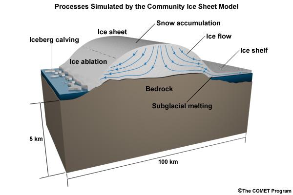
Dynamical ice sheet models simulate the mass and movement of ice that forms on land. Land ice has proven more difficult to model than other aspects of the climate system. While ice generally moves slowly, glaciers and ice shelves can react swiftly under some circumstances. Understanding what can trigger these rapid changes is crucial to projections of sea level. If all the ice in Greenland and Antarctica melted, sea level could rise about 70 meters. The resulting influx of fresh water would likely disturb ocean circulation, further changing climate.

Model Tuning

Why We Tune Models

When we simulate the climate system, we often want to run models for a very long time. For meaningful results, we want no intrinsic drift in global climate. In other words, with constant boundary conditions, the simulated atmosphere/ocean/land system should neither warm nor cool over a long period (except for internal variability). If the amount of energy coming in equals that going out globally, there will be no tendency for the model to drift, to warm or cool. It will be in a steady state, resulting in a stable global control climate.

In a process akin to calibrating laboratory instruments to reduce measurement errors, modelers “tune” the model to achieve a steady state under constant boundary conditions. Once a stable control is established, only then can they design experiments to answer questions about the effects of changing those boundary conditions.

This interactive figure shows one way in which climate models can be tuned to achieve a stable climate. Adjusting the relative humidity threshold for cloud formation, one can increase or decrease the incoming solar radiation that is reflected back to space. If there is too little cloud cover, less incoming solar radiation will be reflected back to space, allowing too much solar radiation reaching the surface. As a result, the model climate will warm. With a long enough simulation, that system will eventually reach a new balance, but the resulting climate will be very warm.

NWP modelers investigating new operational NWP models also test, tune, and retest the models until the skill score of a new model is the same as or better than that of the old model.

How We Tune Models

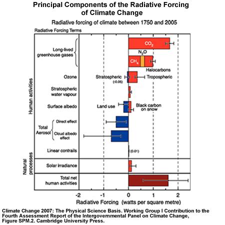
How do we balance the incoming and outgoing radiation to achieve a stable control climate? Usually modelers find a parameterization that has a large effect on the energy budget within the range of observational uncertainty. For example, this graphic shows the change in magnitude of different forcing mechanisms since the start of the industrial era, along with their associated uncertainty.

More typically, modelers choose a parameterization associated with cloud cover. Because clouds reflect solar radiation back to space, the amount of cloud cover strongly regulates the global energy budget. More clouds reflect more sunlight, cooling the Earth. Less clouds allows more sunlight to reach the surface, warming the Earth. We only have rough estimates of the amount of liquid and ice in clouds, the rate at which cloud particles are converted to precipitation, and the impact of clouds on short- and longwave radiative transfer. This allows some latitude in tuning the cloud parameterization to maintain energy balance for a fixed climate model system.

Within the range of uncertainty, parameters within the cloud scheme are adjusted to yield a more realistic energy budget. For example, the rate at which water vapor is converted to cloud water or ice and eventually to rain is not well-understood, with significant uncertainty. If less vapor is eventually converted to rain, then more vapor remains in the atmosphere contributing to cloud formation. Alternatively, more vapor converted to rain tends to dry out the atmosphere, resulting in fewer clouds overall.

Several important points need to be stressed about model tuning:

Tuning is done only within the statistical, physical, or dynamical uncertainty of the parameter. As our understanding of atmospheric processes increases, the uncertainty in parameterizations decreases, making it more difficult to tune models.
Tuning is done to achieve a stable control climate, not to reduce biases in model simulations. We reduce model bias by improving parameterization schemes and/or increasing model resolution.
Tuning is not confined to climate models. Weather forecast models are also tuned, though in a different way.

With weather forecast models, energy balance will have little effect over the short duration of a forecast period. Instead, forecasters may find that the timing or spatial distribution of a specific event is poorly simulated. It could be rainfall amounts or frontal passage associated with storm systems. So, in contrast with climate modelers, forecasters tune weather models to reduce known biases. This is done by experimenting with different parameterizations to identify the source of the bias. For example, model developers may find that the convection parameterization is biased. By changing parameters in the convection scheme, or even replacing the convection scheme altogether, the model may do a better job of simulating a specific type of event.

Both the climate and weather forecasting communities tune their models. They’re tuning them to improve them, and the tuning is done within the range of uncertainty that exists in the observations.

Testing Climate System Models

Model Skill

Once a climate model is tuned and running, it can be tested and evaluated, much as weather models are. In both cases, model results are compared to observations. And, in both cases, model skill has improved significantly over the past thirty years.

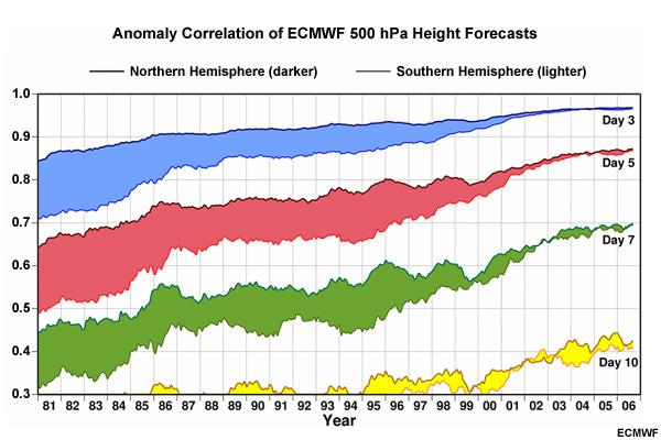
Looking first at weather models, this figure from the European Centre for Medium-Range Forecasts (ECMWF) shows forecast skill for their medium-range NWP model since 1981. It depicts skill (measured by the anomaly correlation) of the 500-mb height forecast for 3, 5, 7, and 10-days in advance. The top line in each color band is skill in the Northern Hemisphere, and the bottom line is skill in the Southern Hemisphere.

Two things are immediately apparent in the graph:

Model skill has increased over the years. For example, if you look at a 5-day forecast, model skill has improved from about 0.60 to about 0.87 (where 1.0 is perfect correlation) over 30 years.
The model has until recently, been much more skillful in the Northern Hemisphere.

This difference in model skill resulted from better initial conditions for weather forecasts in the Northern Hemisphere than the Southern Hemisphere. Until recently, there were more observations in the Northern Hemisphere. Now, satellite data is optimized and the initial conditions have the same quality.

Note that while forecast skill has improved over the last 30 years, the trend has flattened out since about 2003. This could be due to a variety of reasons, including uncertainties in the initial conditions, parameterization biases, and inherent weather predictability issues resulting from internal atmospheric dynamics (i.e., chaos).

Climate models have skill scores similar to those for weather models.

This graphic shows a skill score for successive generations of the atmospheric model component at NCAR over the past 30 years. It is based on the 200-mb height field for the Northern Hemisphere and calculated as one (1) minus the mean square error normalized to the variance of the analyzed observations. The data show that skill has climbed steadily from the very low skill score of the original Community Climate Model (CCM0) in the early 1980s. But, similar to weather forecast models, the skill score for climate models also seems to be flattening out. It is possible that we may reaching some kind of limit on how skillful these kinds of models can be.

Bias in Model Means

SST

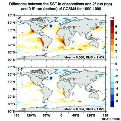
Another way we can test climate models is to look at the spatial distribution of bias in the mean model fields. These plots show the bias in simulated sea surface temperatures from a fully coupled model, the Community Climate System Model compared to the observed SST climatology. The top plot is for a coupled system where the atmospheric model is run at a nominally 2 degree resolution, about two hundred kilometers. The bottom plot is for the same system, but we have increased the atmospheric model resolution to 0.5 degree, including the winds forcing the ocean model. The dynamics and physical parameterizations remain unchanged.

Why?

Higher horizontal resolution increased temperature gradients, which increased the strength of winds in these regions. This increased upwelling of cold water to the surface, reducing the warm temperature bias.

Note the large cold bias in the North Atlantic. It’s still there even in the 0.5 degree model.

Why?

Because it appears that this bias isn’t sensitive to the resolution of the atmospheric model, it is likely due to ocean processes. Preliminary experiments have shown that a much higher resolution ocean model would allow the ocean model to simulate a turnaround of the Gulf Stream as it approaches Greenland. With this turn, the Gulf Stream warms these regions, eliminating the cold bias.

Sea Ice

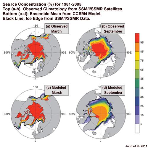
The Arctic is an interesting place to examine model biases because the climate exhibits strong feedback due to the high albedo of snow and ice. These plots show sea ice concentration and extent from satellite observations and the CCSM4 climate model for the period 1981-2005. The annual sea ice maximum typically occurs in March, while the annual sea ice minimum typically occurs in September.

Precipitation

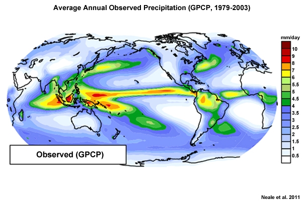
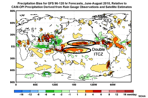
Biases still remain in climate models. One in particular is the so-called double Intertropical Convergence Zone, or ITCZ, bias in precipitation. In general, coupled climate models show excessive tropical precipitation, which through ocean-atmosphere coupling, leads to less precipitation in the equatorial Pacific. A drier equatorial bias splits the wetter tropical Pacific into northern and southern bands, giving rise to the apparent double ITCZ.

Comparing the bias for the 1-degree and 2-degree versions of the model, we can see that increasing the model resolution has only a small effect on the bias. Biases like the double ITCZ motivate researchers to improve the parameterization schemes that lead to excessive tropical precipitation.

Note that NWP models produce similar biases. This graphic shows biases produced by GFS 4-5 day forecasts for June through August, 2010. Even over this brief period, a double ITCZ is apparent, along with excess precipitation in the Himalaya. These and other features are similar to those we saw in long-term simulations by climate models.

Biases in Initialized Climate Models

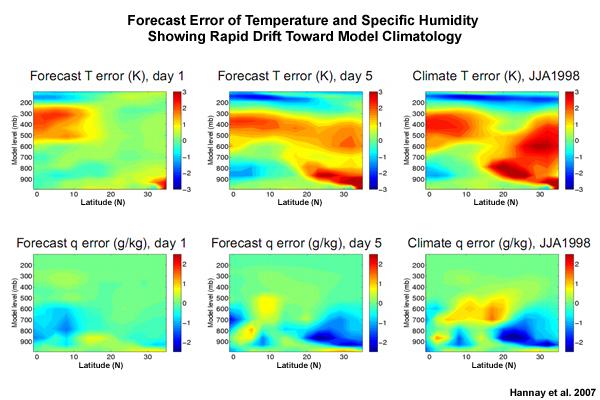
Another way to examine climate model bias is to run the model as a forecast model. This has been done by initializing the climate model, not from observations, but rather from re-analysis products. After running the model for several days, researchers can examine how biases develop as the simulation drifts away from the observed climatology toward the model’s steady-state climate.

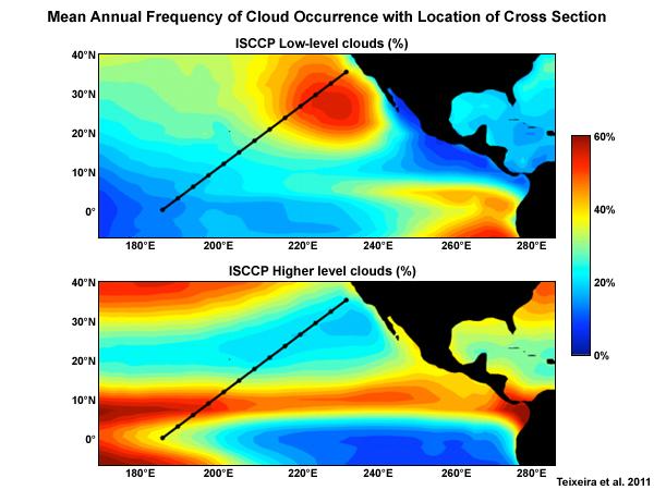
In these simulations, researchers were looking at the bias in tropospheric moisture and temperature over a transect from San Francisco out to the Equatorial Pacific. Along this transect, the cloud regime goes from low marine stratus near the California Coast to deep convection near the Equator. Thus, this transect provides a way to examine biases in a variety of cloud processes.

Note: ISCCP = International Satellite Cloud Climatology Project

The results are startling. These plots are vertical cross sections of model bias relative to observed climatology for 1 day (left), 5 days (center), and the long-term climate model mean (right). The top row of plots shows temperature, while the bottom row shows moisture.

What you see, is that bias starts to build immediately and within 5 days the forecast bias in temperature looks very similar to the long-term climate bias. Similarly, the dry bias seen in the climatology near the coast in the lower troposphere shows up in the forecast after 5 days.

This experiment provides researchers with a very powerful tool for research. Why?

It takes a lot of computer time to run climate models for 10, 20, or 100s of years to look at biases. If the same bias shows up in a 5-day initialized forecast, it enables us to very quickly analyze biases due to physical parameterizations. We no longer have to run the model for decades or centuries to look at some of the biases related to different physical parameterizations. Rather, we track down the source of the bias using a series of 5-day forecasts!

This experiment also very clearly shows how weather forecast models will drift if they aren’t re-initialized frequently to keep pulling them back to observations. Model simulations drift very quickly into their own biased state. Weather forecasters know this from looking at longer runs of weather forecast models.

Natural Variability

North Atlantic Oscillation

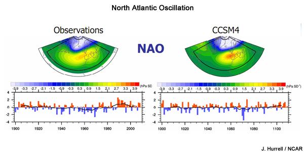
Climate statistics encompass more than just the mean state for climate. They also include measures of natural variability, including the location, timing, and strength of oscillations within the climate system. For example, fully coupled models generate variability on the same time and spatial scales as ENSO, the North Atlantic Oscillation (NAO), and Pacific Decadal variability, among others.

This is a plot of one mode of variability found in the climate system, the North Atlantic Oscillation (NAO), which is a pressure oscillation between the Arctic region and the subtropics. The plot on the left shows the annual mean NAO in the real atmosphere from 1900 to 2008, while the plot on the right shows the annual mean NAO in a fully coupled model over a 109-year period. The results are strikingly similar.

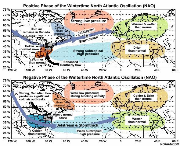
It’s important to note that this variability is not externally forced. This is a natural mode of variability of the Earth’s climate system that happens to play a very important role for seasonal weather. Here we see typical global weather patterns associated with positive and negative modes of NAO.

From 2008 to 2011, a tendency toward a strongly negative phase of NAO resulted in extremely cold winters in Europe. Having a climate model generate this sort of variability is important because that variability goes into the statistics of weather that comprise climate for the Northern Hemisphere.

ENSO

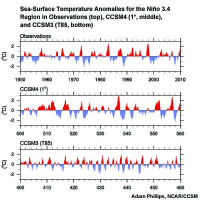
A similar argument can be made for ENSO. We know that ENSO plays a very important role in seasonal weather phenomena, especially in tropical regions and some extratropical regions, especially in the cold season. Therefore, getting a good simulation of ENSO leads to a more realistic climate simulation and more robust climate statistics. This plot of SST anomalies shows the improvement in both the magnitude and periodicity of ENSO variability between the older CCSM3 and newer CCSM4 simulations.

Overall, it’s very important to get a climate model that is not just simulating mean temperature and moisture distribution, but also simulating these various modes of variability.

Future Directions

Increased Model Complexity

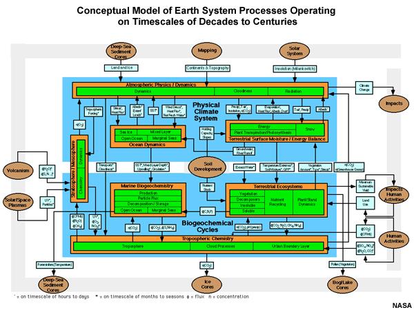
About 30 years ago, Francis Bretherton developed this system flow chart of the Earth’s climate and biospheric cycles, which has forever become known as the Bretherton diagram. When seeing this diagram for the first time, the first reaction of many people is laughter: the diagram is so very complex. It’s got everything. It’s got human impacts, it’s got volcanism, it’s got space physics, it’s got deep sea sediment cores, and the solar system. Bretherton put everything in. This diagram could be seen as a model roadmap; Bretherton’s grand view of where models would need to evolve. Indeed, they have been evolving in this direction over the last 20 years.

One of the more significant additions from early efforts has been the inclusion of ecosystem models. This includes a terrestrial ecosystem component in the land model along with a marine ecosystem component in the ocean model.

Why include ecosystems?

Most of the climate models of the last 20 years have specified the amount of carbon dioxide in the atmosphere, not predicted it. It was prescribed based on very good measurements of carbon dioxide, but there has always been a goal to make carbon dioxide a predicted quantity. To do that, models need to simulate the carbon cycle. Now many models are being run that do not prescribe the amount of carbon dioxide in the atmosphere. Instead, only emissions of carbon dioxide due to the burning of fossil fuel are set. Then the model calculates how much carbon dioxide remains in the atmosphere.

In addition to simulating the processes that make up the carbon cycle, models now include chemistry that impacts atmospheric gas composition, as well as aerosols and clouds. Adding complexity to models, like atmospheric chemistry, ecosystems, and the carbon cycle, lets the model do what the real climate system is doing: exchanging not only moisture and energy between the surface and the atmosphere, but also carbon dioxide.

Increased Model Resolution

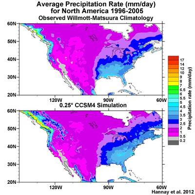
The other revolution in climate simulation is increased model resolution. As computers have gotten more and more powerful, models are able to be run at higher and higher resolution. These plots show mean annual precipitation for North America in mm/day. The top plot comes from an observational data set over a 10-year period. The bottom plot shows results from an atmospheric model run at a quarter-degree grid spacing, using actual SSTs to capture the model response to processes like ENSO. That’s equivalent to about a 25-km grid box size, the same as many weather forecast models. We can now run global models over decades to centuries at the same spatial resolution as forecast models. And as we can see here, models are beginning to capture not just the large, general features of precipitation, but even details down to small scales.

And models have been run down to even finer resolution. One of these images is the result of a climate model initialized with observations, like a forecast model, and run at 5-km resolution to simulate a particular storm system. The other image is the satellite observation of the actual storm system.

So not only are models getting more complex, but there is a parallel path wherein models are being run with increasing horizontal resolution, in both the atmosphere and the ocean. In general, the more we increase resolution, the more improvement we see in the model simulations. However, not all model fields are improving with increased resolution, and increasing resolution further may not yield significant improvement. Biases still remain, but many are now clearly related to parameterization schemes.

The Goal

Eventually climate and weather modelers would like to merge increased resolution and added complexity and run the most complete models at 10 to 20 km resolution with the most accurate parameterization schemes.

There are still biases in models. There will always be biases in models. But the models are grounded in basic physics and they’re tested against multiple data sets of observations, in terms of both the mean and the variability. Thirty years ago atmosphere-only models were run with prescribed sea surface temperatures. Now we’re running fully coupled Earth system models for thousands of years, and the models keep getting better.

Summary

The modeling of both weather and climate share a deep history and common pedigree based on fundamental laws of physics. The key difference between climate and weather models lies not in the models themselves, but in the questions they seek to answer. Weather models predict how weather will evolve from an initial state for a particular place and time. Climate models project how the statistics of the climate system will respond to changes in external forcing (i.e., boundary conditions).

For the climate system to be in a steady state, the long-term average energy coming in must balance the long-term energy going out. Boundary conditions in climate models affect the way that energy is absorbed or exchanged in the climate system. Boundary conditions are not predicted by the model and must be specified. Boundary conditions include solar radiation, atmospheric composition, and land use.

Atmospheric and oceanic circulation develops in response to the unequal distribution of incoming solar energy across the globe. Climate models have to account for these circulations. To directly simulate processes in Earth’s climate system, models use a set of equations that balance forces acting in three dimensions and conserve mass and track the temperature of each grid layer. These are the resolved processes.

Processes that operate on a scale smaller than the model grid must be parameterized. That is, their effect over the entire grid cell is given by a single value. Examples include the latent heating due to cumulus convection or the radiative transfer of solar and longwave radiation.

The components that go into a climate model include an atmosphere model, ocean model, land model (including snow and land ice), and sea ice model. A coupler manages the interactions between the different components, accommodating different grids, resolution, and time steps.

When we simulate the climate system, we want no intrinsic climate drift in the model. In a process akin to calibrating laboratory instruments, modelers “tune” the model to achieve a steady-state. To tune a climate model, modelers vary a parameterization that has a large effect on the energy budget within the range of observational uncertainty.

Climate models can be tested in several ways.

We can develop skill scores, which reduce model biases to a single number.
We can examine the spatial and temporal distribution of biases in model means.
We can compare the natural variability in the simulated climate with that in the observed climate.

In the future we expect that increasing computational capabilities will allow models to be run at increased resolution and complexity. As model complexity increases, more parameters become predicted, rather than prescribed. The eventual goal of climate and weather modelers is to run the most complete models at high resolution with the most accurate parameterization schemes.

References

Climate Change 2007: The Physical Science Basis. Working Group I Contribution to the Fourth Assessment Report of the Intergovernmental Panel on Climate Change, Figure SPM.2. Cambridge University Press.

Hannay, C., D. Williamson, J. Olson, J. Hack and J. Kiehl, R. Neale and C. Bretherton (2007), Sensitivity to the CAM candidate schemes in climate and forecast runs along the Pacific Cross-section, CCSM Atmosphere Model Working Group (AMWG) Meeting, 29-31 January 2007, NCAR, Boulder, Colorado www.cgd.ucar.edu/cms/hannay/publications/AMWG2007.pdf

Hannay, C., R. Neale, and J. Bacmeister (2012), High Resolution Climate Simulations with the Community Atmospheric Model (CAM), AMS 92th meeting, New Orleans, 22-26 January 2012. www.cgd.ucar.edu/cms/hannay/publications/AMS2012.pdf

Jahn, A., and Coauthors, 2012: Late-Twentieth-Century Simulation of Arctic Sea Ice and Ocean Properties in the CCSM4. J. Climate, 25, 1431–1452. http://journals.ametsoc.org/doi/abs/10.1175/JCLI-D-11-00201.1

Landrum, L., B. L. Otto-Bliesner, A. Conley, P. Lawrence, N. Rosenbloom, and H. Teng. Last Millennium Climate and Its Variability in CCSM4. *Journal of Climate Special Issue Collection on CCSM4 *http://www.cesm.ucar.edu/publications/jclim10/docs/landrum.ccsm4.last_millennium.pdf

Lawrence, D.M., K.W. Oleson, M.G. Flanner, P.E. Thornton, S.C. Swenson, P.J. Lawrence, X. Zeng, Z.-L. Yang, S. Levis, K. Sakaguchi, G.B. Bonan, and A.G. Slater, 2011: Parameterization improvements and functional and structural advances in version 4 of the Community Land Model. J. Adv. Model. Earth Sys., 3, DOI: 10.1029/2011MS000045. http://james.agu.org/index.php/JAMES/article/view/v3n1

Neale, R. B., J. Richter, S. Park, P. H. Lauritzen, S. J. Vavrus, P. J. Rasch, and M. Zhang. The Mean Climate of the Community Atmosphere Model (CAM4) in Forced SST and Fully Coupled Experiments. J. Climate, in press. http://www.cesm.ucar.edu/publications/jclim10/docs/ccsm4.html

Pongratz, J., C. Reick, T. Raddatz, and M. Claussen (2008), A reconstruction of global agricultural areas and land cover for the last millennium, Global Biogeochem. Cycles, 22, GB3018. http://www.agu.org/journals/gb/gb0803/2007GB003153

Teixeira, J., and Coauthors, 2011: Tropical and Subtropical Cloud Transitions in Weather and Climate Prediction Models: The GCSS/WGNE Pacific Cross-Section Intercomparison (GPCI). J. Climate, 24, 5223–5256. http://journals.ametsoc.org/doi/abs/10.1175/2011JCLI3672.1

Trenberth, K.E., J.T. Fasullo, J. Kiehl, 2009: Earth’s global energy budget. Bull. Amer. Meteor. Soc., 90, 311–323. http://journals.ametsoc.org/doi/abs/10.1175/2008BAMS2634.1

Trenberth, K.E., J.M. Caron, 2001: Estimates of meridional atmosphere and ocean heat transports. J. Climate, 14, 3433–3443. http://journals.ametsoc.org/doi/abs/10.1175/1520-0442%282001%29014%3C3433%3AEOMAAO%3E2.0.CO%3B2

Willis, J. K., D. Roemmich, and B. Cornuelle (2004), Interannual variability in upper ocean heat content, temperature, and thermosteric expansion on global scales, J. Geophys. Res., 109, C12036, doi:10.1029/2003JC002260. http://www.agu.org/pubs/crossref/2004/2003JC002260.shtml

Earth-system climate modeling – historical perspective

GCM future climate datasets

Note that the IPCC’s goals, as stated above in this chapter, do not explicitly include the mandate of providing future change model outputs and data sets that would be useful, say, for this primer’s user audience (aka needed to drive more local scale impact models). However, with this said, both the IPCC’s Data Distribution Centre (DDC) and CMIP’s ``Program for Climate Model Diagnosis and Intercomparison <https://pcmdi.llnl.gov/>`__ (PCMDI) at Lawrence Livermore National Laboratory have been supporting access to data sets that would be useful for the audience, with the PCMDI ESGF Portal being a well-used portal for acquiring dynamical downscaling data sets. Also, NCAR also has its CMIP Analysis Platform (https://www.cisl.ucar.edu/computing-data/data/cmip-analysis-platform) that gives researchers convenient access to climate data from CMIP, along with direct access to other related NCAR model data dealing with climate change. Two examples are the CESM Large Ensemble Community Project (LENS; https://www.cesm.ucar.edu/community-projects/lens) and the follow-on LENS2 (https://www.cesm.ucar.edu/community-projects/lens2),`publicly available sets of climate model simulations intended for advancing understanding of internal climate variability and climate change through the generation of many ensembles starting from initial starting points in the atmosphere (LENS and LENS2) and ocean (just LENS2). This initialization design is intended to enable an assessment of oceanic and atmospheric contributions to ensemble spread (i.e. the natural variability of the Earth system), and the impact of initial-condition memory on the global Earth system.

One word of caution: the historic period GCM CMIP6 outputs to these models are provided so that researchers can assess the GCM skill at reproducing the general statistical behavior of the Earth system, including trends and potential biases in this behavior. However these data are not designed to be compared with specific historic events (e.g. a specific year’s and region’s heat wave or flooding event), since the models’ states are started from an observed initial state, but then are free to internally equilibrate, with only certain historic forcings providing the models with further constraints as they run forward over the historic period. The constraining forcings are:

Greenhouse Gases: Concentrations of CO2, CH4, N2O, and other greenhouse gases.
Aerosols and Ozone: Historical data on aerosols (such as sulfate, black carbon, organic carbon) and ozone concentrations.
Land Use Changes: Historical land use and land cover changes, including deforestation, urbanization, and agricultural practices.
Solar and Volcanic Activity: Variations in solar irradiance and major volcanic eruptions.

Note that this lack of constraints on the GCMs over the historic period is in contrast to how these same GCMs might be used to produce reanalysis data sets over the historic period, where model states are continually brought back to be consistent to observations collected over the period.