Chapter 5: Baseline natural variability and attribution of observed changes

This Chapter provides an overview and guidance on the following topics:

• Characterizing baseline natural variability and introduction to the attribution of observed changes

Table of Contents

• Key takeaways from the chapter

• Introduction

  • Weather and climate

  • Natural factors influencing climate variability

• Baseline natural variability and detection and attribution of observed changes

• References

Attribution

Much of the material and images used in this chapter are derived from the following MetEd Lessons: Preparing Hydro-climate Inputs for Climate Change in Water Resource Planning; Climate and Water Resources Management, Part 1: Climate Variability and Change; Climate and Water Resources Management, Part 2: General Principles in Integrating Climate Change; Climate Change and Extreme Weather. The source of this material is the COMET® Website at http://meted.ucar.edu/ of the University Corporation for Atmospheric Research (UCAR), sponsored in part through cooperative agreement(s) with the National Oceanic and Atmospheric Administration (NOAA), U.S. Department of Commerce (DOC). ©1997-2024 University Corporation for Atmospheric Research. All Rights Reserved.

Chapter 5 Key Takeaways

Detection is the identification of a significant change in the climate system (temperature, precipitation, wind patterns, shifts in seasonal cycles, etc.) that is above and beyond the natural internal variability of the system.

Climate attribution deals with determining the causes of detected changes in the climate. This involves assessing the various natural and anthropogenic (human-induced) factors that could have led to the observed changes.

Attribution of observed changes is not possible without some kind of model of the relationship between external climate drivers and observable variables, given that we cannot observe a world in which neither anthropogenic or natural forcing exist.

• Such models may be very simple (e.g., a set of statistical assumptions) or very complex (e.g., coupled Earth System Model)

A more recent approach in climate modeling for detection and attribution is to run a “Large Ensemble” of historical (and future) simulations, where each member of the ensemble is subject to natural+anthropogenic external forcings, but starts from a slightly different initial condition, which results in a different trajectory of internal variability once the memory of the initial state is lost.

The following observed and/or projected trends have an impact on planning for water and environmental resources:

• Global average temperature has been warming and will continue to warm through the 21st century

• Short-term natural cycles of increased warming interspersed with cooling (or slower warming) will be superimposed on the overall long-term warming

• Average snow cover and snowpack in the United States are likely to decrease through the 21st century

• Precipitation extremes (wet and dry) are likely to continue increasing through the 21st century, with some regional trends toward either more wet or more dry

• These climate trends have, and will continue to have, impacts on water resources

5.1 Introduction

In this chapter we discuss the concept of the baseline natural variability of a system under study, and ways to detect and potentially attribute the contribution of observed changes to natural and anthropogenic factors. Because climate change is a phenomenon that is typically characterized by slow changes through time, and that anthropogenic-induced climate change predominantly began in the mid-19th century (when atmospheric concentrations of CO2 began to show a marked increase correlating with industrial activities), significant changes may be detected through examination of the historical record, depending on the study area. At the same time, detection depends on how large the “natural variability” of the system of interest is. The Earth’s climate systems exhibit natural variability due to a range of factors. These include variations in solar radiation (e.g., solar cycles), volcanic activity, ocean currents, atmospheric circulation patterns such as El Niño and La Niña, and geological processes like the shifting of tectonic plates (at time-scales of millions of years). Additionally, feedback mechanisms within the Earth’s climate system can amplify or dampen these variations, leading to fluctuations in temperature, precipitation patterns, and other climatic parameters over different timescales, from years to centuries and beyond. The figure below from the Intergovernmental Panel on Climate Change (IPCC: https://www.ipcc.ch/report/ar6/syr/figures/figure-2-1) shows (on the left panel) the increase in the global surface temperature through time, while the panel at the right shows estimates of how much these temperature changes have been attributed to total human influence; solar and volcanic drivers; and internal climate variability. Although at the global scale, human impacts are the dominant contributor to these changes, natural variability generally becomes relatively a much larger contributor to observed changes as the spatial region of interest gets smaller, and as the timescales of interest also decrease.

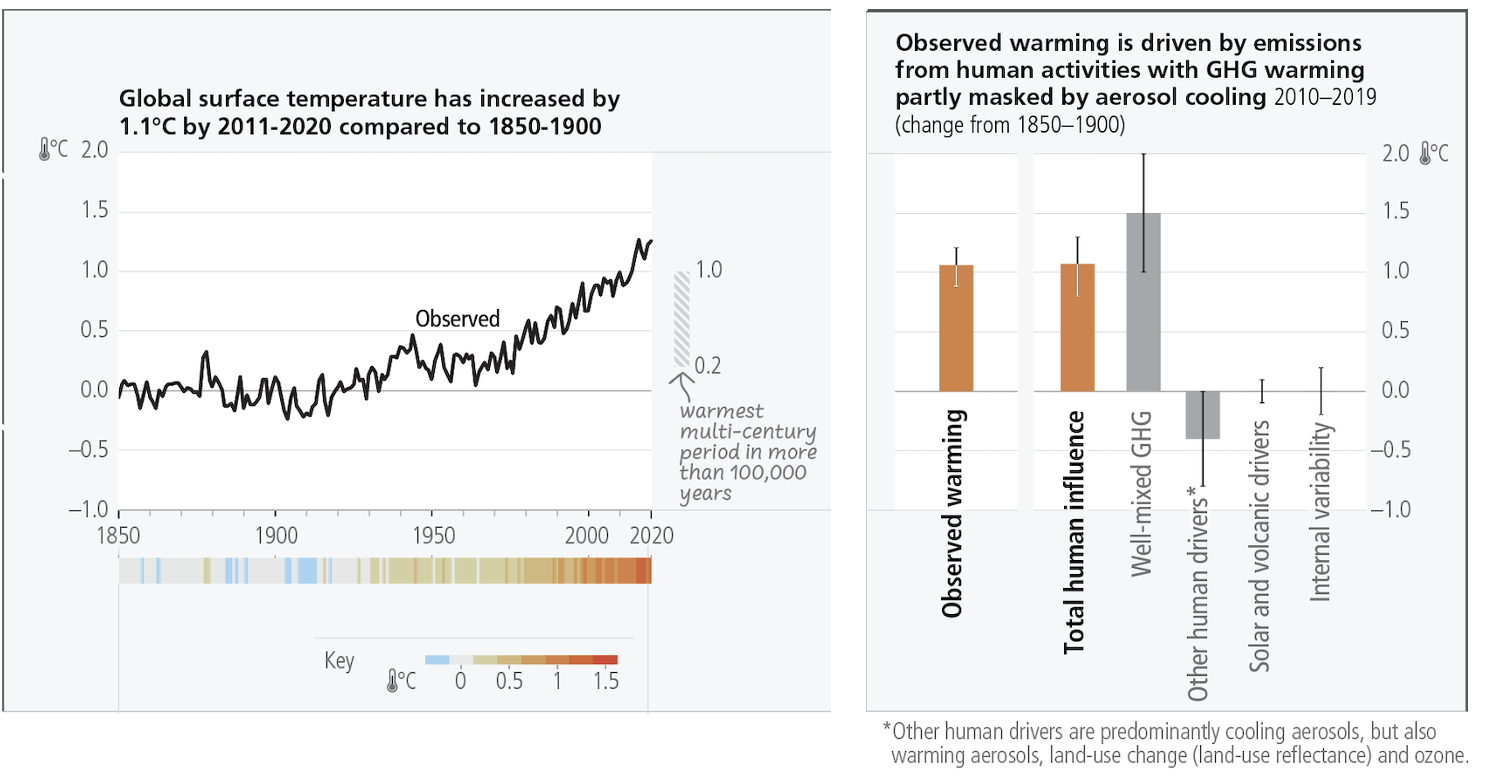
Figure:Left panel: the global surface temperature (shown as annual anomalies from a 1850–1900 baseline) has increased by around 1.1°C since 1850–1900. Right panel: temperature change attributed to: total human influence; its decomposition into changes in greenhouse gas (GHG) concentrations and other human drivers (aerosols, ozone and land-use change (land-use reflectance)); solar and volcanic drivers; and internal climate variability. Whiskers show likely ranges. Source: IPCC: https://www.ipcc.ch/report/ar6/syr/figures/figure-2-1.

We start with a brief overview of what these different types of variability are, where they have already been observed, then discuss methods that can be more generally applied to a particular region to discern these different types of variability.

Here we provide introductory background information.

The pop-out below discusses the distinction of weather and climate (i.e., differences in what are often termed “time scales of interest”).

Weather vs Climate

Most of us know that climate and weather are not the same. It is sometimes said, “Climate is what you expect, weather is what you get.”

Weather describes the details of what we experience over the course of hours and days.

Climate is the statistical representation of weather over days, months, seasons, years, decades, and longer

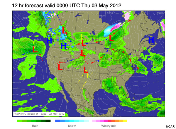
A weather prediction, or forecast, describes the near-term likelihood of a weather event such as a specific occurrence of rain or snow and/or the expected change in temperature. A weather forecast, for example, might read “colder with a 70% chance of snow this afternoon.”

A climate prediction, on the other hand, might call for below-average precipitation and near-average temperature over the next 30 days.`

Climate-model output: used to generate statistics of weather phenomena`

-Mean and variability of precipitation and temperature

-Collective impact of weather events

Projections: Lack specificity and predictability

Climate models do predict specific weather events many years into the future, but not with the intention for use as time- and site-specific forecasts. Rather, the intended use of climate-model output is to generate statistics of weather phenomena, such as means and variability of precipitation or temperature, to characterize the collective impact of weather events. These climate predictions are typically referred to as projections or simulations and lack the short-term specificity of weather predictions.`

The pop-out below provides a description of the natural factors that influence our climate over time.

Natural factors impacting climate variability

Earth’s climate shifts over time because so many different land, ocean, and space phenomena have influence. The sun is the main driver of Earth’s climate, as it provides most of the energy. The sun’s energy output increased about a tenth of a percent from 1750 to 1950, which contributed about 0.2°F (0.1°C) warming in the first part of the 20th century. But since 1979, when we began taking measurements from space, the data show no long-term change in total solar energy, even though Earth has been warming.

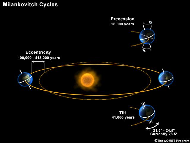
Repetitive cycles in Earth’s orbit can influence the angle and timing of sunlight. The tilt and wobble of Earth’s axis and the degree to which its orbit is stretched produce the Milankovitch cycles, which scientists believe both triggered and rewarmed ice ages for the last few million years. But these changes take thousands of years, and so cannot explain the warming in this century.

[Click to open a drifting continents & ocean currents animation.](https://www.meted.ucar.edu/broadcastmet/climate/media/video/continents_currents.mp4)

Drifting continents make a big difference in climate over millions of years by changing ice caps at the poles and by steering ocean currents, which transport heat and cold throughout the ocean depths. In turn, these currents influence atmospheric processes. Snow and ice on Earth also affect climate because they reflect more solar energy than darker land cover or open water.

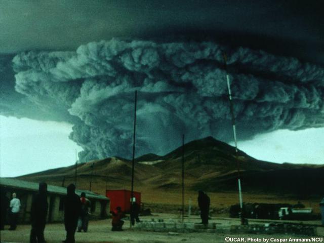
Huge volcanic eruptions can cool Earth by injecting ash and tiny particles into the stratosphere. The resulting haze shades the sun for a year or two after each major blast. Dust and tiny particles thrown into the air by both natural processes and human activities can have a similar effect, although some absorb sunlight and help heat the climate.

Greenhouse gases, which occur both naturally and as a result of human activities, also influence Earth’s climate.

The pop-out below provides background information on the Earth’s energy balance, the factors that influence it, and thus lead to climate variability and change.

Earth’s energy balance and the greenhouse effect

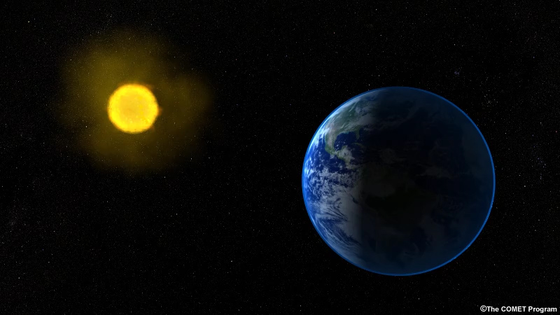
The Earth is in a delicate equilibrium of solar energy (mainly shortwave ultraviolet) entering and longwave energy (mainly infrared) leaving. Slight alterations to this balance impact weather and climate. These can be caused by the natural cycles of climate variability, such as volcanic eruptions, that temporarily reduce the amount of solar energy reaching the Earth’s surface, thus disrupting the energy balance.

Small changes to the balance of energy between the Sun and Earth are driving recent trends in global temperature.

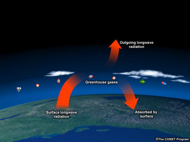
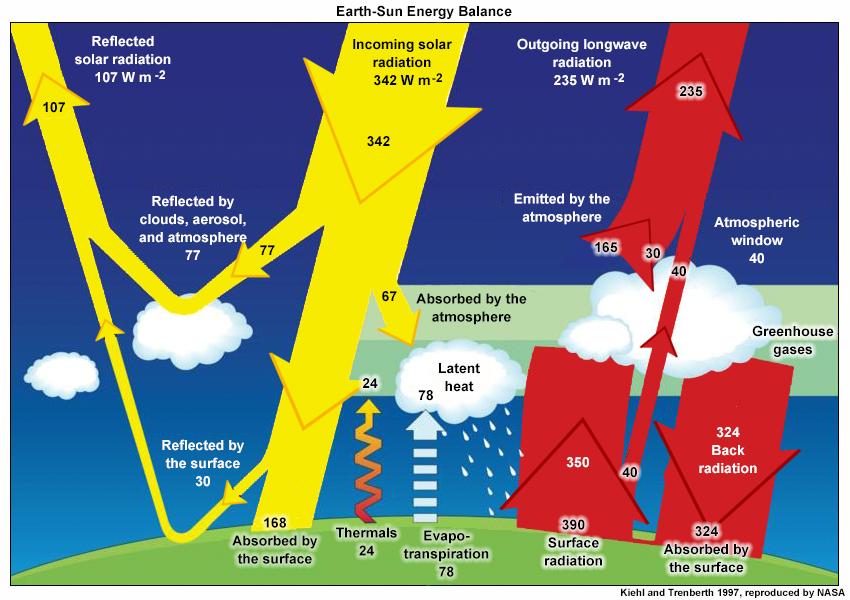
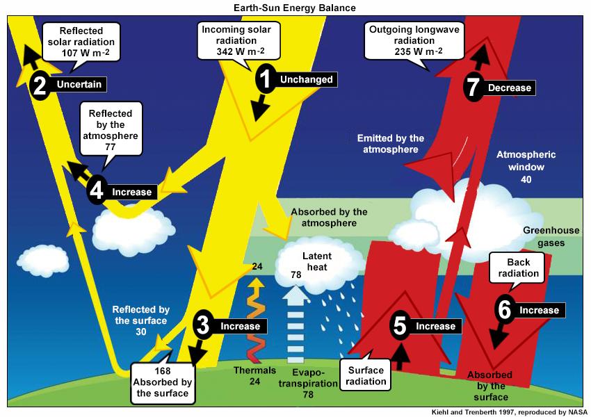
The diagram below of the energy cycle shows the amount of energy, in Watts per square meter, that enter the Earth-atmosphere-ocean system, remains within it, and leaves. Notice that about one third of the 342 W/m2 of solar energy (the yellow arrows) is reflected back to space by the atmosphere or surface, while about two thirds are absorbed. As we’ve seen, the magnitude of solar energy reflected by aerosols sometimes increases temporarily after major volcanic eruptions, leading to temporary decreases in solar energy reaching Earth’s surface.

On the right side of the diagram, the red arrows show the amount of terrestrial energy (mainly infrared) emitted by the Earth’s surface and atmosphere. Some is radiated back to space. But due to the presence of greenhouse gases, carbon dioxide, and water vapor in particular, a significant portion is absorbed by the atmosphere and re-radiated back to Earth. The “Back Radiation” portion of the diagram shows the heat energy radiated from the atmosphere to the surface. This is the Greenhouse Effect. Without naturally occurring greenhouse gases, the Earth would be an inhospitably cold and frozen planet.

The pop-out below provides introductory information on natural climate variability versus anthropogenic climate change examples for streamflow, CO2 emissions, and global temperature anomalies.

Introductory information

Scientists have explored past global temperature trends using proxy data—tree rings, ice cores, etc.—that show the Earth has had numerous and somewhat irregular swings in temperature over the past several hundred thousand years. Those swings in temperature contribute to variations in other natural phenomena such as streamflow.

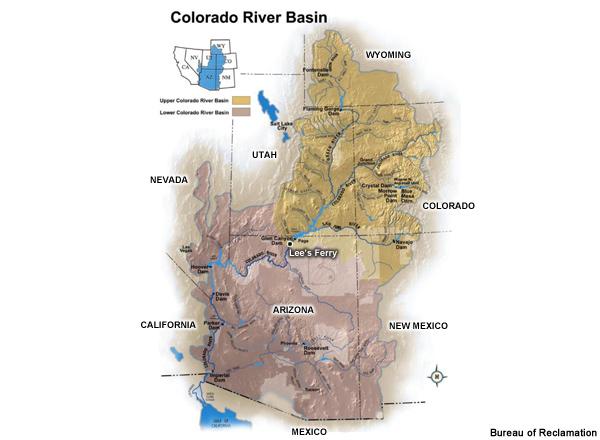
For example, tree-ring analysis can be used to reconstruct streamflow in the rivers of the western United States. This has been done for rivers such as the Colorado River at Lee’s Ferry, in the state of Arizona.

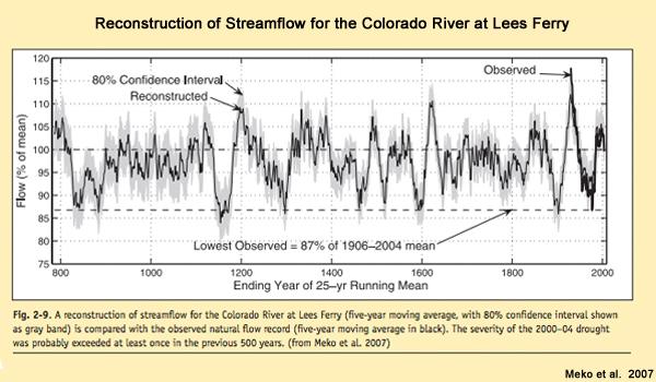
The reconstructed streamflow shows large swings in annual streamflow volume on the Colorado River. Multi-year periods of wet and dry can be seen in the 25-year running mean of the annual streamflow.

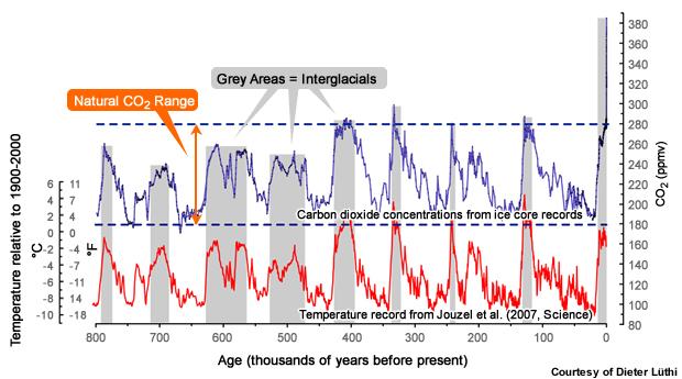
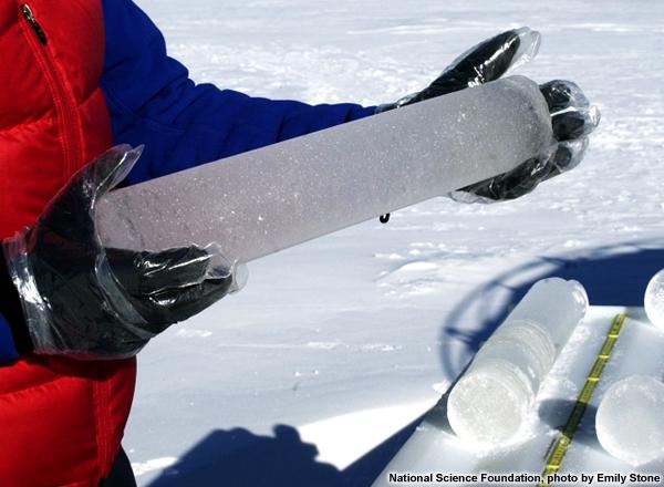
Ice cores, on the other hand, can provide a depiction of changes in global temperature and CO₂ levels over the past several hundred thousand years. This graphic shows that warmer periods coincide with higher levels of CO₂.

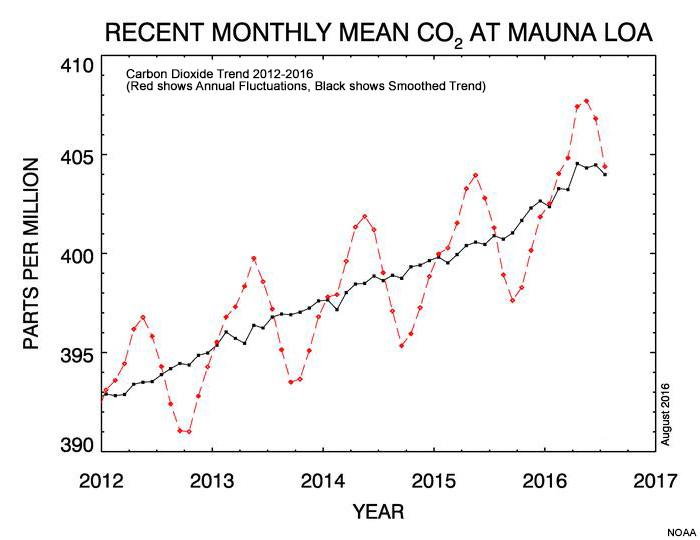
Carbon dioxide levels have naturally fluctuated between 180 parts per million (ppm) and 280 ppm. This is an example of a naturally occurring climate forcing. Human industrialization has been a major source of the increase in CO₂ in the most recent century, with average annual concentrations exceeding 420 ppm in 2024. This is an example of anthropogenic forcing. We can see how carbon dioxide concentration has continued to rise over the last decade, as seen in the black line in the figure below.

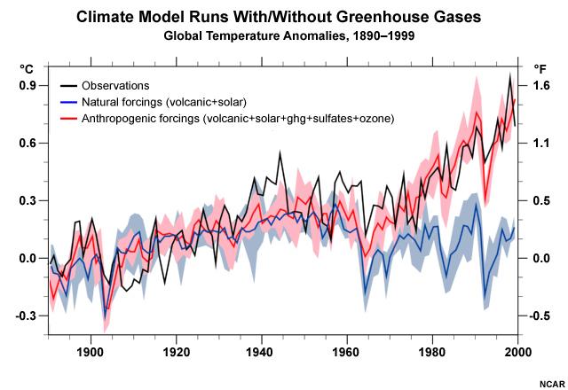
Trajectories of past global mean temperatures have been estimated using experiments conducted with Atmosphere-Ocean General Circulation Models (AOGCMs). Experiments that do not incorporate anthropogenic forcing produce the trajectory shown with the blue line and the light blue uncertainty bounds in the figure below.

The black line shows the observed global mean temperatures. You can see that the experiments that do not include anthropogenic forcings fail to reproduce the warming that has been observed over the past half century.

Experiments were also run that do include anthropogenic forcings. This trajectory is shown with the red line and pink uncertainty bounds. You can see that when anthropogenic forcings are included, the global climate models do produce results that very closely match the observed warming trends. This suggests that anthropogenic factors have emerged as a significant contributor to global warming.

5.2 Climate variability

When accounting for climate-change impacts on research in water and environmental studies, it is important to differentiate between climate variability (for which the past can be a guide) and climate change, where the past is not necessarily a good predictor as climate change involves changes to this natural variability. Starting off this section, we will review some of the natural climate cycles and occurrences.

Regular climate cycle

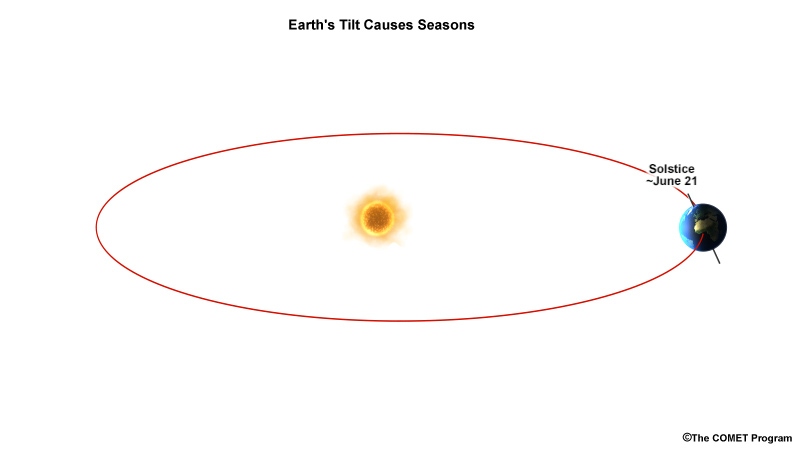
The most regular climate cycle is the change of seasons. The seasons determine the times of year when precipitation may be most abundant, evapotranspiration will peak, tropical cyclones are most likely to form, and snowpack accumulates and melts. Although the change of seasons is very dependable, there is often year-to-year variation.

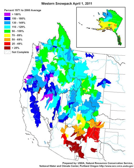
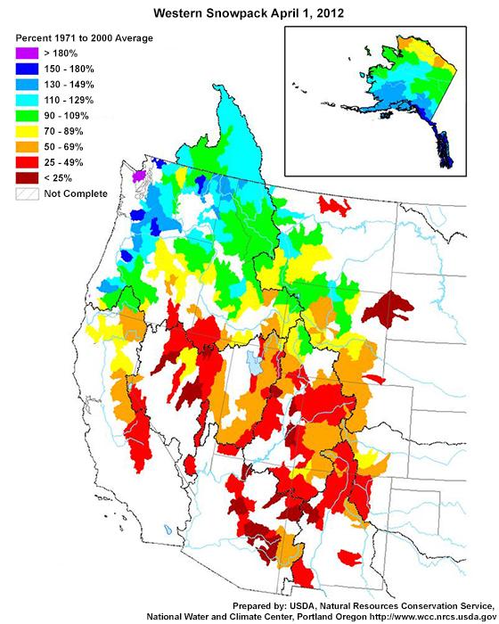
To illustrate natural season-to-season variability, here we see differences in snowpack on the first of April in two consecutive years. The 2011 analysis shows large areas with above average snowpack in the central Rocky Mountain region and California Sierra Nevada Range in the United States. In 2012, these same areas had abnormally low snowpack, reflecting a less abundant snow season. Good research planning allows for such variation. But will the expected range of snowpack change as the climate warms?

When speaking of climate change, we are referring to changes in average weather conditions that persist over multiple decades or longer. Climate change encompasses both increases and decreases in temperature, as well as shifts in precipitation, changes in frequency and location of severe weather events, and changes to other features of the climate system.The principal natural drivers of climate change (which are also termed “external natural forcings”), include changes in incoming solar radiation (through solar cycles), volcanic activity, orbital cycles, and changes in global biogeochemical cycles.`

Irregular climate impacts

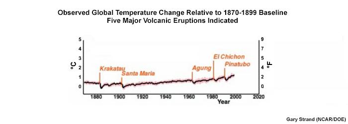
Major volcanic eruptions are irregular natural climate events. In this global temperature time series, we can see how the sun-shielding properties of atmospheric aerosols from volcanic eruptions result in decreased global average temperatures. Notice how Mt. Pinatubo’s 1991 eruption decreased global average temperatures for 1-2 years.

Very long-term climate variability

There are much longer climate variability cycles associated with changes in the Earth’s orbital eccentricity and its tilt with respect to the Sun.

These cycles, known as the Milankovitch Cycles, lead to big changes in the amount and distribution of solar energy on the Earth’s surface. The global temperature during these long-duration cycles ranges from being much colder (the ice ages) to much warmer than the current global average temperature.

Milankovitch Cycles unfold on timescales much longer than a human life span, from tens to hundreds of thousands of years. The rate of change associated with the Milankovitch Cycles is so slow that it will not impact water research planning for the next century or so.

Major anthropogenic drivers include atmospheric aerosols (fine solid particles or liquid droplets), land-use change, and CO2 and non-CO2 greenhouse gases. The natural and anthropogenic drivers taken together make up what are called climate forcings.

Climate forcings

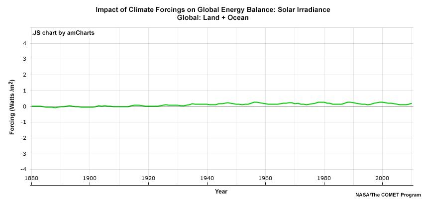
In this pop-out, we will examine how a number of forcings (both natural and anthropogenic) have influenced the energy balance between the Earth and Sun from 1880 to 2014, determining whether each forcing has had a warming effect (in which case the forcing goes above the zero change line) or a cooling effect (in which case the forcing goes below the zero change line).

Solar irradiance leads to some cyclic warming, but has a very small magnitude.

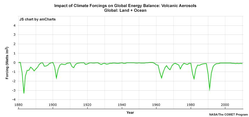
Volcanic eruptions have a notable cooling impact due to increased atmospheric albedo triggered by reflective volcanic aerosols. The cooling from volcanoes in the period examined was temporary, never lasting more than a few years. And, they had no real impact on the long-term trend.

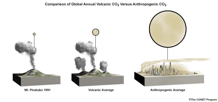
What effect does a typical large volcano have on carbon dioxide

concentration compared to the effect from human activity? The diagram shows that in a typical year, the CO2 emissions from anthropogenic sources is 135 times greater than those from volcanoes, with some studies showing even greater differences. Even the 1991 eruption of Mt Pinatubo put roughly 1/500th of the 2010 emissions from anthropogenic activity into the atmosphere.

Now we’ll look at the Land-Use Forcings. What impact does land use have on the solar energy absorbed at the Earth’s surface?

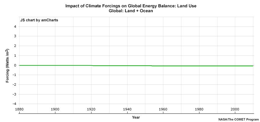
Land use leads to very small decreases in the energy absorbed at the surface, or small amounts of cooling. That’s because replacing forests with agricultural or urban land tends to increase the surface albedo and reflect more solar energy back to space.

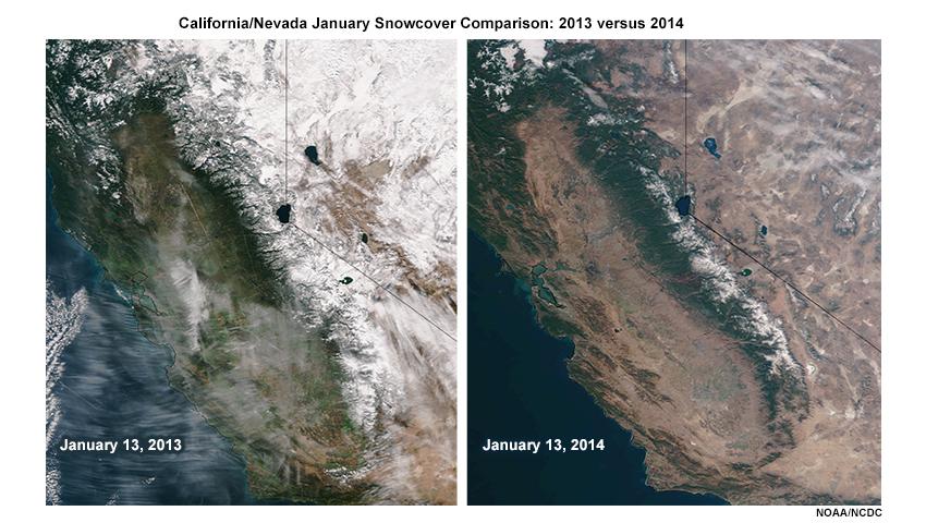
Albedo is a measure of how well a surface can reflect solar energy. Reflective surfaces, like snow, ice, and clouds, have high albedo and are efficient at reflecting solar energy back to space. In the satellite images centered on the Sierra Nevada, snow and clouds have very high albedo and appear white. You can see that there may be large year-to-year differences in snow cover and thus the albedo. Even desert sands have high albedo and show up as relatively bright in this visible satellite imagery.

Dark-colored surfaces have low albedo and absorb solar energy. This impacts the solar energy absorbed by Earth. Forest areas appear dark on visible satellite images, and are more efficient at absorbing solar energy. Bodies of water appear very dark and have very low albedos.

Now we’ll look at the impact of Anthropogenic Aerosols (those resulting from human activity). What kind of impacts are related to anthropogenic aerosols?

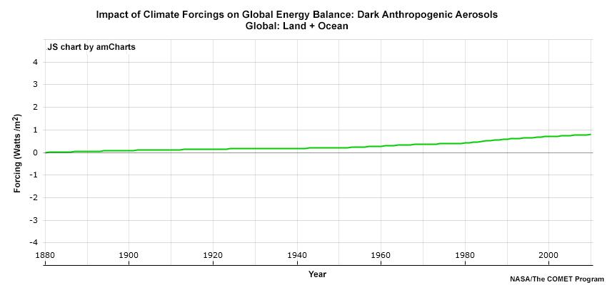
Anthropogenic aerosols have both warming and cooling impacts. That’s because different aerosols have opposite effects on albedo. Dark particulates, such as black carbon, decrease albedo and increase absorption of solar energy, resulting in a warming effect. This occurs in the atmosphere as a whole, but also when black carbon settles out on otherwise reflective surfaces, such as snow and ice.`

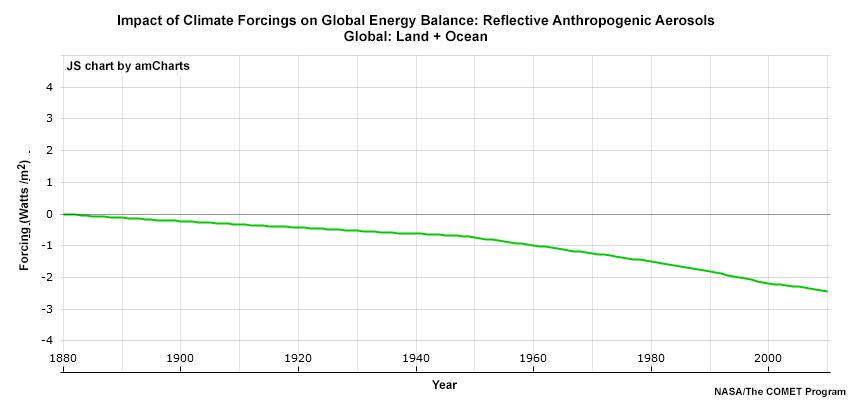
Other aerosols in the atmosphere are reflective and increase atmospheric albedo. This can occur from the aerosols themselves reflecting sunlight back to space, or from aerosol enhancement of cloud development (an indirect effect). Cloud tops have high albedo and reflect solar energy back to space.

What has the overall impact of anthropogenic aerosols been?

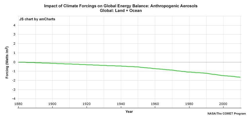
The reflective anthropogenic aerosols dominate and thus the impact of all anthropogenic aerosols leads to climate cooling.

Now we’ll look at the impact of Greenhouse Gases. All of the greenhouse gases result in a warming trend. Well mixed gases, such as carbon dioxide, methane, and nitrous oxide, have the greatest impact, and this impact is increasing with time.

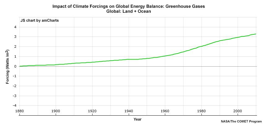
The magnitude of the warming from greenhouse gas forcing is greater than the notable cooling effect from reflective aerosols.

Now we’ll look at all forcings combined.

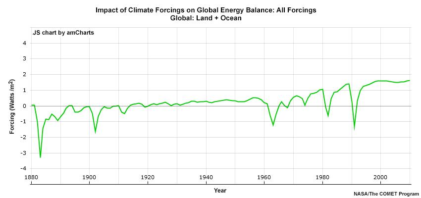
When all variables are included in one time series, the trend induced by greenhouse gas forcing is clear. Net climate forcing has increased by 1 to 2 Watts per square meter since pre-industrial times, leading to the warming of the Earth by 1ºC (1.8ºF) through 2015. The warming effect induced by greenhouse gases has been tempered by the overall cooling effect of anthropogenic aerosols, and occasional short-duration cooling from volcanic aerosols.

As we’ve seen, anthropogenic climate forcings result in a steady trend in global warming, with short-term variations caused by natural factors. Anthropogenic forcings have led to both global cooling (from reflective aerosols) and warming (from greenhouse gases) but the warming dominates over periods of multiple decades or longer.

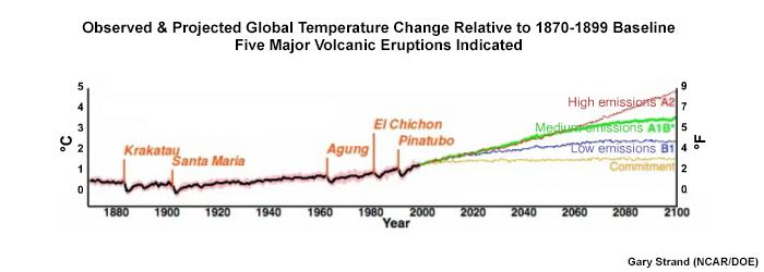
By the middle part of the 21st century, even the cooling impact from notable volcanoes like Krakatau and Pinatubo won’t be able to temporarily cool the average global temperature to average 20th-century levels according to climate model projections.

When viewed in the context of Earth’s average temperature over hundreds of thousands of years, the current warming is on par with some past epochs. But the increase in carbon dioxide, the most abundant anthropogenic greenhouse gas, is much greater than in past warm periods. This suggests that our very rapid warming–and it is very rapid on the geologic time scale–is just beginning. This greenhouse gas-induced warming is likely to dwarf the cooling factors as we move through the 21st century.

The pop-out below discusses how the components of the energy cycle are expected to change over the next few decades based on anthropogenic changes to specific forcings.

Climate forcings impact on energy balance

In this pop-out we discuss how the components of the energy cycle are expected to change over the next few decades based on anthropogenic changes to specific forcings (discussed in previous pop-outs), while assuming continued emissions of greenhouse gases:

• Incoming solar radiation (1) should stay the same over the time period of decades.

• Total reflected solar radiation from Earth (2 and 4) is uncertain. Increases in reflected solar energy are likely given that reflective aerosols and/or cloud cover continue to increase. But the uncertainty is because surface albedo should decrease with the continued loss of snow and ice.

• The amount of solar energy absorbed at the ground is uncertain. Of the solar radiation that reaches the surface, a greater proportion is likely to be absorbed (3) due to the continued loss of snow and ice, but increases in reflective aerosols and clouds could reduce the amount of solar energy reaching the ground.

• As the global land and ocean surfaces (5) continue to warm on average, the radiative energy from the surface should continue to increase.

• Increasing greenhouse gases (6) will likely increase the amount of terrestrial radiation that is radiated back to the surface.

• The longwave radiation leaving the Earth (7) should decrease because more is being trapped by the atmosphere.

• It is important to note that the answers for all of the longwave fluxes could be different if rapid emissions reduction occurs.

In addition to these secular changes to the climate, there is also variability that originates from natural processes within the coupled ocean-atmosphere-cryosphere-land-biosphere system that is generally termed internally generated variability, arising primarily from the uneven distribution of energy across the planet at any given time (Lehner and Deser, 2023). A primary source of internal variability is the atmospheric general circulation with its day-to-day and week-to-week weather fluctuations with limits to their predictability past a couple of weeks, and can be termed random or stochastic processes past those limits. In general, the climate system is highly variable at regional scales, and this internally-generated variability is irregular in time and exhibits limited predictability. Processes arising from the coupling between the ocean and atmosphere are also important sources of internally generated variability that give rise to distinctive patterns (or “modes”) of variability on interannual and longer timescales (Deser and Phillips 2023). Examples include the interannual events of El Niño Southern Oscillation (ENSO); and the Pacific Decadal Oscillation (PDO) and the Atlantic Multidecadal Oscillation (AMO) patterns which can influence regional climate conditions, such as droughts or cooling periods. It is a central scientific challenge to identify anthropogenic influences on weather and climate amidst this background of internal variability (Deser et al. 2020).

Semiregular climate cycles`

Recurring, but less regular, climate cycles often have a large influence on how the seasonal climate variations play out.

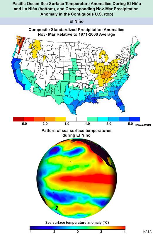
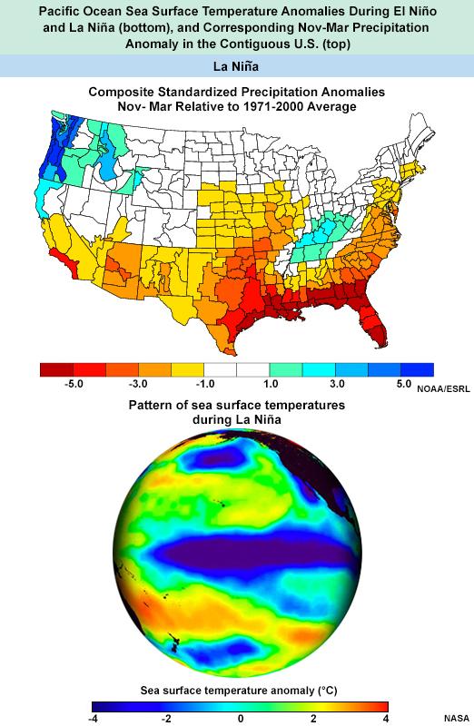
A well known, semi-regular climate cycle is associated with the El Niño Southern Oscillation (ENSO). ENSO can have a significant impact on precipitation and temperature in many regions of the world in a cycle that recurs roughly every 3-4 years.

In the contiguous United States, the ENSO cycle can significantly influence precipitation distribution, especially in the cool season.

Below we see the typical impacts of El Niño versus La Niña on both the sea-surface temperature anomalies of the tropical Pacific Ocean, and the November through March precipitation in the contiguous United States. The difference can be very important for snowpack and the potential for regional floods and drought. There are differences from one cycle to the next, but these composite maps provide guidance based on historic data. Note that La Niña typically results in a drier winter across a broader area than El Niño.

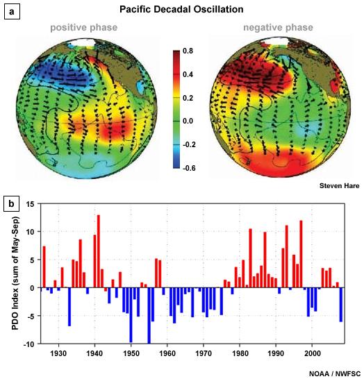
Like ENSO, there are other natural atmospheric and oceanic cycles that have regional impacts on precipitation and temperature, including the Pacific Decadal Oscillation (PDO), as seen below. And like ENSO, local research planning typically considers the range of variations that these cycles cause.

Natural climate variability can temporarily obscure or intensify anthropogenic climate change on decadal time scales, especially in regions with large internal interannual-to-decadal variability. Both the rate of long-term change and the amplitude of interannual (year-to-year) variability differ between global, regional and local scales, between regions and across climate variables, thus influencing when changes become apparent. As an example, tropical regions have experienced less warming than most others, but also exhibit smaller interannual variations in temperature. Accordingly, the signal of change is more apparent in tropical regions than in regions with greater warming but larger interannual variations (IPCC WG1).

The relative influence of natural and anthropogenic-induced variability is also dependent on the spatial scale of the system being examined. In general, the signs of climate change are unequivocal at the global scale but are more difficult to discern on smaller spatial scales. Discernible changes also depend on the climate variable. For example, changes in average rainfall are becoming clear in some regions, but not in others, mainly because natural year-to-year variations in precipitation tend to be large relative to the magnitude of the long-term trends.

The case study in the pop-out below of surface temperature changes over time provides a visualization of natural variability and its sensitivity to spatial and temporal scales, along with sensitivity and detection of secular anomalies and trends.

Natural variability case study

This case study provides a visual sense for the natural variability in long-term temperature trends across time scales and spatial scales, and the discernment of significant changes outside of this natural variability. Shown in the two figures below are the surface-temperature trends since 1880 comparing the observed temperature record of two domains: 1) “Global: Land + Ocean” (first figure) and, 2) “Global: Land Only” (second figure). The blue line in the graph depicts the global mean annual temperature anomalies from 1880 to 2014. An “anomaly” is simply the departure of a temperature from a baseline, in this case the average temperature. For example, if the average temperature for today is 15°C but the actual temperature is 18°C, then the temperature anomaly is +3°C. If the actual temperature was 12°C, then the anomaly would be -3°C. In these two times series, the anomalies are based on the 30-year average from 1951-1980. Therefore, the anomalies show the departure of each average annual temperature from that 30-year average. The red line represents the trend for the entire 1880-2014 period. You can see year-to-year variability in the anomalies, as well as variability on the decadal time scale.

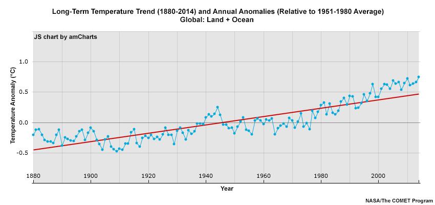
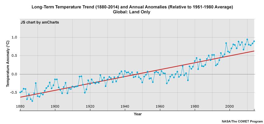
The overall warming trend (red line) for “Global: Land Only” is a bit steeper than “Global: Land + Ocean”. The “Land Only” trend shows more than a +0.5°C departure from the mean by 2014, while the “Land + Ocean” trend shows a little less than a +0.5°C departure. Due to the oceans’ ability to store heat, the global warming trend is a bit slower when they are included. This, then, also highlights the dependence of land-temperature variability on its proximity to large water bodies.

Below we highlight the dependence on the variability to (smaller) spatial scale, showing the trend for the Contiguous United States.

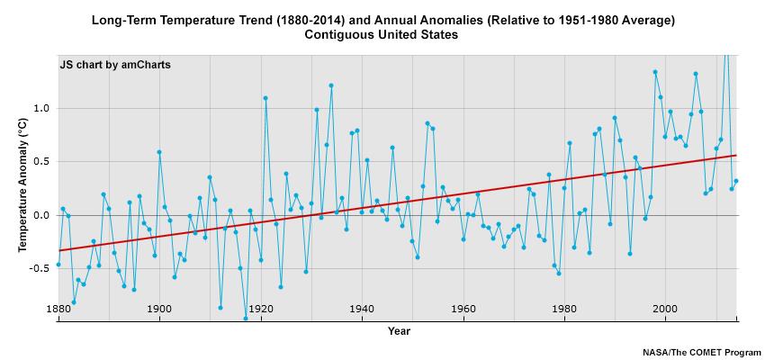
The “Contiguous United States” trend shows a little less rapid warming than the “Global: Land Only” areas, but the year-to-year variability is much greater. Generally, the variability will continue to increase as the spatial domain covered decreases. The 48 contiguous states make up only 1.6% of the global surface and are not, by themselves, a good measure of global trends.

Next we focus on the dependence of trend on time period, and again examine the “Global: Land + Ocean” domain (shown below). If we were to fit 10-year trend lines over differing periods of this record, one would find 10-year periods with upward, downward, and no trend in temperature. For example, the decade of 1941-1950 shows distinct cooling, while the overlapping decade of 1933-1942 shows very distinct warming. Since the mid-20th century, 10-year temperature trends are mainly warming, although there are flat periods as well as year-to-year variation (noting that the last 10-year period shown in the graph below, 2005-2014, has no trend but is warmer than every other 10-year period in the 20th century). Internal variability drivers are the predominant mechanisms for this year-by-year, decadal-by-decadal trend variability and the motivation to “smooth over” this variability is one reason why both the World Meteorological Organization (WMO) and the National Oceanic and Atmospheric Administration (NOAA) accept 30 years as the period of time used to define a climate station’s “climate normals”. Note that one of the “climate-normal” periods is shown below covering 1938-1967.

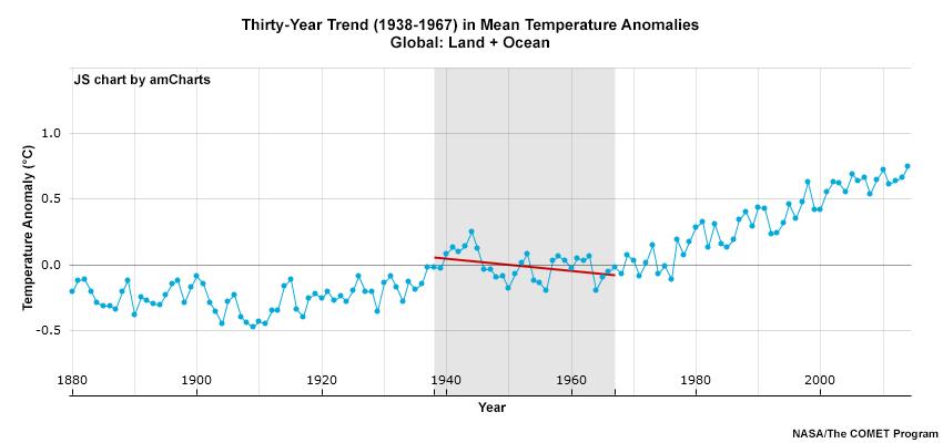
Interestingly, during this 30-year period (1938-1967) the global surface temperature actually decreased by about 0.1°C, and was caused by sulfate particles from the increased burning of fossil fuels backspattering to space, and was thus a cooling anthropogenic climate driver. However, this trend stopped once the United States and other countries began to lower sulfur emissions in the 1970s to reduce acid rain and respiratory illnesses (since 1975, the average global temperature has risen by about 0.15-0.2°C per decade). This observed cooling effect is one reason why the injection of sulfate aerosols into the upper atmosphere is actively being considered as one mechanism of geoengineering to limit global warming.

5.3 Detection and Attribution

Detection and Attribution is a complex scientific discipline, so below we provide only an overview of this field along with some of the more common detection and attribution approaches, and refer the reader to the following resources for more detailed information (the latter three from which we draw much of the material presented below):

• The International Detection and Attribution Group (IDAG; http://www.image.ucar.edu/idag/ and http://www.clivar.org/clivar-panels/etccdi/idag/international-detection-attribution-group-idag), an international group of scientists who have collaborated since 1995 on assessing and reducing uncertainties in the estimates of climate change.

• Contribution of Working Group I to the Sixth Assessment Report of the Intergovernmental Panel on Climate Change (IPCC, 2021), Chapter 1 (Chen et al., 2021), Chapter 3 (Eyring et al., 2021), Chapter 10 (Doblas-Reyes et al., 2021), and Chapter 11 (Seneviratne et al., 2021).

• The Fourth National Climate Assessment Volume I (USGCRP, 2017), Chapter 3 (Knutson et al., 2017) and Appendix C (Knutson, 2017).

• The National Academies of Sciences, Engineering, and Medicine. 2016. Attribution of Extreme Weather Events in the Context of Climate Change (NAS, 2016)

Detection – Detection and attribution are two important concepts in the field of climate science, particularly when studying climate change. Detection refers to the process of demonstrating that some aspect of climate has changed in some statistical sense, without providing a reason for that change. It is about identifying a significant change in the climate system (temperature, precipitation, wind patterns, shifts in seasonal cycles, etc.) that is above and beyond the natural internal variability of the system. Detection does not imply understanding the cause of changes; it’s about observing (or making a determination beyond a level of significance) that a change has occurred, and provides the basis for attributing these changes to specific causes, such as human activities. Because of the presence of natural variability and other noise in the data under study, distinguishing a climate-change induced signal is more often a statistical process (e.g., a detectable observed change is one that is determined to be highly unlikely to occur – say, less than about a 10% chance – due to internal variability alone).

The popout below provides an overview of the changes in climate-variable statistical distributions that could result from climate change. In context of detection, there are a variety of statistical tests that can be used to test the significance of differences between distributions (e.g., the Kolmorgorav-Smirnov two-sample test that two data samples come from the same distribution; NIST 2023; Chakravart et al. 1967; Press et al. 1992).

Climate change and extremes

Just as changes in annual and seasonal mean temperature and precipitation are very important to water research and resources, depending on the particular focus of the planning, changes in short-duration extremes can be very important too. Extremes can directly impact habitat, and pose risks to infrastructure. It is important to get a sense for what extremes represent from a statistical standpoint. Extreme weather is a bit relative. For example, a hot day in Wyoming would be considered a mild one in Arizona. And we don’t generally notice changes in climate because most weather falls within the range of what is expected. It is mainly the extreme events that get our attention—events that are outside our normal experience and that often inflict human suffering. So how might global warming affect climate extremes and extreme weather? There are several possible ways.

Temperature at a given location can be roughly represented with a bell curve or a normal distribution, similar to the top panel in the figure below, with the majority of the observations in the middle, hot and cold events in the tails of the curve, but with rare events of extremely cold or extremely warm temperatures at the ends. Global warming could shift the distribution to the right when the average temperature increases. Temperatures that used to be unusually high become more common, while heat levels not reached before become more probable. Cold extremes still occur, but become less common. Although not shown here, a:mark:`nother possibility is that climate change increases the variance (or width) in the distribution of temperature—in other words, it increases the range of possibilities at both ends of the distribution. Or climate change could result in a combination of the two types of distributions. We don’t a priori know exactly how the distributions of weather variables in each specific location will be influenced.

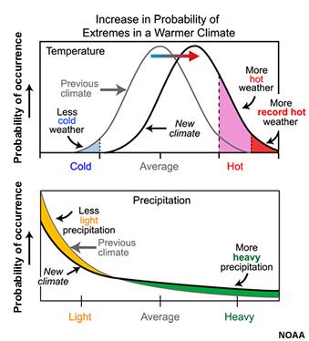
Precipitation curves have only one tail for the extreme precipitation events, as shown in the bottom panel of the figure above (with the two-parameter gamma traditionally used; Ye et al. 2018). In a warmer climate with more atmospheric water vapor, generally, more intense precipitation events become more common. Recent observations back this up, with high-end precipitation events becoming less rare than they have been, in general.

Attribution – On the other hand, attribution deals with determining the most likely causes for those detected changes in the climate. This involves assessing the various natural and anthropogenic (human-induced) factors that could have led to the observed changes, with these often complex, interacting factors that can range in scales from molecular to global, seconds to millennia. Attribution studies can use statistical tests as well as climate models, to evaluate the relative contributions of various causes to climate change (along with an assignment of statistical confidence), like greenhouse-gas emissions, solar radiation, and volcanic activity, with the latter (coupled climate models) being an especially powerful tool with potential to turn on and off factors in controlled numerical simulations of the areas and events of interest. A supporting concept is the idea of emergence of a climate change signal or trend, referring to when a change in climate (the “signal”) becomes greater than the amplitude of natural or internal variations (defining the “noise”) (AR6). This concept is often expressed as a “signal-to-noise” ratio (S/N) and emergence occurs at a defined threshold of this ratio (e.g. S/N >1 or 2) (Chen et al. 2021).

Elements of a Detection and Attribution Study – The AR6 Cross-Working Group Box on Attribution (Hope et al. 2021) provides a brief discussion and figure (reproduced below), on Steps towards an attribution assessment; and a similar discussion on four core elements to any detection and attribution study is also provided in AR5 WG1 (Bindoff et al. 2013: 10.2.1 The Context of Detection and Attribution). Taken together, the following general steps are identified: a) the unambiguous framing of what changes are being attributed to; b) clearly define the indicators of the observed change or event, including observations of one or more climate variables, such as surface temperature, that are understood, on physical grounds, to be relevant to the process in question, and note the quality of the observations; c) the identification of the possible and plausible drivers of change, including an estimate of how external drivers of climate change have evolved before and during the period under investigation, including both the driver whose influence is being investigated (such as rising greenhouse gas levels) and potential confounding influences (such as solar activity); d) the development of a hypothesis or theory for the linkage with a quantitative physically based understanding, normally encapsulated in a model, of how these external drivers are believed to have affected these observed climate variables; e) and a system or method to test the hypothesis or theory, typically including an estimate, often but not always derived from a physically based model, of the characteristics of variability expected in these observed climate variables due to random, quasi-periodic and chaotic fluctuations generated in the climate system that are not due to externally driven climate change.

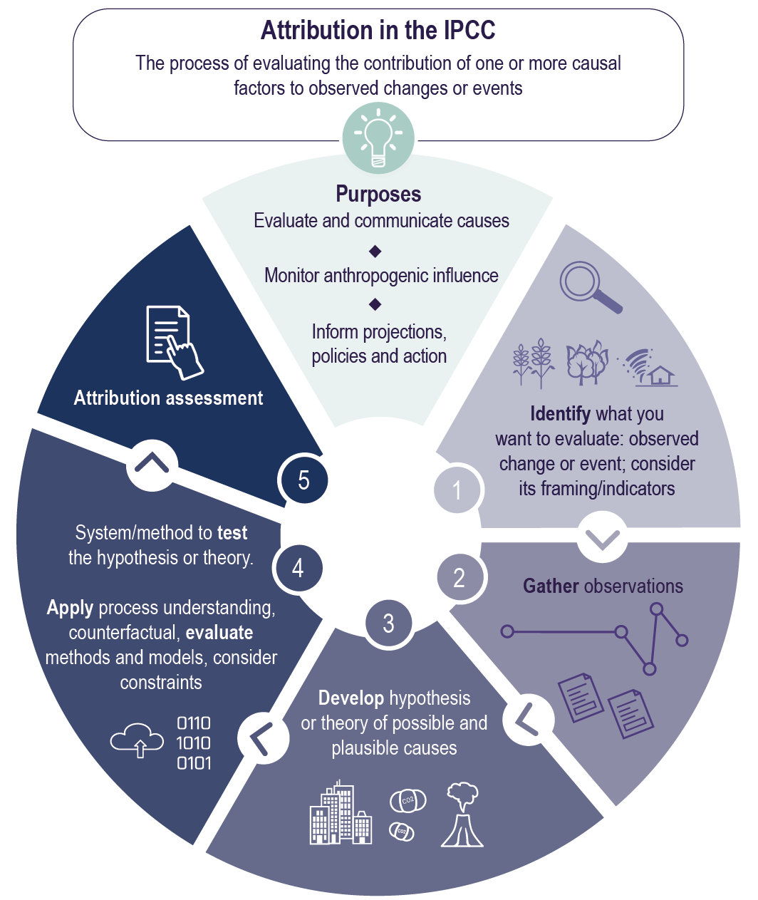
Figure: Cross-Working Group Box: Attribution, Figure 1 | Schematic of the steps to develop an attribution assessment, and the purposes of such assessments. Methods and systems used to test the attribution hypothesis or theory include: model-based fingerprinting; other model-based methods; evidence-based fingerprinting; process-based approaches; empirical or decomposition methods; and the use of multiple lines of evidence. Many of the methods are based on the comparison of the observed state of a system to a hypothetical counterfactual world that does not include the driver of interest to help estimate the causes of the observed response.

Attribution Methods – Concerning the attribution methods or system to test the hypothesis or theory, Bindoff et al. (2013) highlight that the attribution of observed changes is not possible without some kind of model of the relationship between external climate drivers and observable variables given that we cannot observe a world in which neither anthropogenic or natural forcing exist. Such models may be very simple (e.g., a set of statistical assumptions) or very complex (e.g., coupled Earth System Model), and that it is not necessary (or possible) for them to be correct in all respects, but they must provide a physically consistent representation of processes and scales relevant to the attribution problem in question.

Some of the most powerful tools in the attribution process are models of the system of interest that use “what if” approaches to isolate the impacts of anthropogenic (and other) factors that are hypothesized to be driving the changes in the observed record. It is to be noted with very high confidence (IPCC 2021) that the CMIP6 model ensemble reproduces the observed historical global surface temperature trend and variability with biases small enough to support detection and attribution of human-induced warming (Eyring et al. 2021), and that CMIP6 also includes an extensive set of idealized and single forcing experiments for attribution (Eyring et al. 2016; Gillett et al. 2016), but with the important caveat that numerical models, however complex, cannot be a perfect representation of the real world, and their use requires considering the limitations of each model simulation (see 1.5.4 in Chen et al. 2021). The figure below highlights an earlier effort that used the “what if” approach on a global scale, where the impacts of anthropogenic forcings are isolated through the use of NCAR’s coupled Earth System Model. Trajectories of past global mean temperatures have been estimated using experiments that do not incorporate anthropogenic forcing produce the trajectory shown with the blue line and the light blue uncertainty bounds. The black line shows the observed global mean temperatures. You can see that the experiments that do not include anthropogenic forcings fail to reproduce the warming that has been observed over the past half century. Experiments were also run that do include anthropogenic forcings. This trajectory is shown with the red line and pink uncertainty bounds. You can see that when anthropogenic forcings are included, the global climate models do produce results that very closely match the observed warming trends. This suggests that anthropogenic factors have emerged as a significant contributor to global warming.

A more recent approach in climate modeling for detection and attribution is to run a “Large Ensemble” of historical (and future) simulations, where each member of the ensemble is subject to natural+anthropogenic external forcings, but starts from a slightly different initial condition, which results in a different trajectory of internal variability once the memory of the initial state is lost. One can estimate the forced component from the ensemble-average at any point in time, since the internal component is randomly phased across the different members of the ensemble. The figure below (Deser et al. 2020) illustrates how the random phasing of internal variability of 60-year trends over North America can obscure the forced trend at any given location. Note the regional differences in the spatial patterns of the trends over this time period (comparing the coldest and warmest ensemble members for the same model on the bottom row); and by extension, how much greater the natural variability is at these smaller spatial scales. Such Large Ensembles, then, provide context for interpreting observed trends. In this context, the actual observed trajectory can be considered as one realization of many possible alternative worlds that experienced different weather. This can also be demonstrated by the construction of “observation-based large ensembles,” which are alternate possible realizations of historical observations that retain the statistical properties of observed regional weather (e.g. McKinnon and Deser 2018; Chen et al. 2021). Referring back to the concept of signal-to-noise and to the second panel of the figure, the ratio of the mean shift from zero of the distributions (forced signal) compared to (some metric of) their spread (internal variability “noise”) provides a degree of the emergence in the anthropogenically-forced North America heating trend.

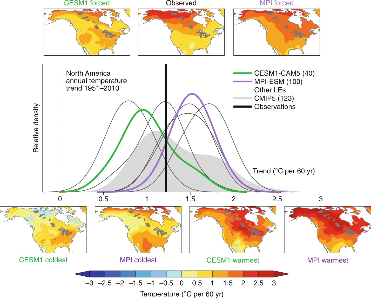
Figure: The distribution of 60-yr annual temperature trends (1951–2010) over North America (24–72° N, 180–62° W) from seven ESM LEs (thin curves), 40 different CMIP5 models (grey shading), and observations (Berkeley Earth Surface Temperature; vertical black line). The maps show the associated patterns of temperature trends: top row, observed and the forced component (estimated by the ensemble mean) from two LEs (CESM1 in green and MPI in purple); bottom row, individual ensemble members from CESM1 (green) and MPI (purple) with the weakest (“coldest”) and strongest (“warmest”) trends. Note that the individual member maps show the total (forced-plus-internal) trends in the model LEs. Observed trends are analogous to an individual ensemble member in that they reflect forced and internal contributions. From: Deser et al. 2020, Nat. Clim. Chang., 10, 277-286, doi:10.1038/s41558-020-0731-2, Copyright 2020 Nature Climate Change.

Generally, attribution methods are grouped into two categories: Attribution of observed climate change to anthropogenic forcing and Attribution of weather and climate events to anthropogenic forcing, as will the discussion that follows. Because the focus of this primer is on climate-change impacts on North America water studies, the focus in what follows will be on regional approaches to this topic, referencing Doblas-Reyes et al. (2021) for the discussion of Attribution of observed climate change to anthropogenic forcing, referencing Seneviratne et al. (2021) for Attribution of weather and climate events to anthropogenic forcing, and we refer the reader to Eyring et al. (2021) for a discussion of the methods used for global-scale studies.

Attribution Methods: Attribution of observed climate change to anthropogenic forcing – Here, regional-scale attribution is the process of evaluating the potential contributions of multiple causal factors (or drivers) to regional climate change. Specific regional conditions and responses may simplify or complicate attribution on those scales. In general, regional climate variations are larger than the global mean climate, adding additional uncertainty to attribution. In contrast with global-scale attribution methods where internal variability might be considered as a noise problem, the preliminary detection step is not always required to perform regional-scale attribution since causal factors of regional climate change may also include internal modes of variability in addition to external natural and anthropogenic forcing. Other complicating factors include an increased similarity among the responses to different external forcings leading to a more difficult discrimination of their effects, the importance of some omitted forcings in global model simulations at regional scale, and model biases related to the representation of small-scale phenomena (Zhai et al. 2018). These statistical limitations may be reduced by process-based (or regional-scale) attribution, focusing on the physical processes known to influence the response to external forcing and internal variability. We provide a summary of these attribution methodologies next, after first noting that these methodologies rely upon the availability of high-quality observational datasets as well as multi-model simulations of the historical period constrained by different external forcing combinations, including single-forcing experiments and single-model initial-condition large ensembles (SMILEs).

Standard approaches include optimal fingerprinting methods that are based on multivariate linear regression and assume that the observed change exhibits a linear combination of externally forced signals plus internal variability. The main goal is to determine the extent to which observed climate changes can be attributed to specific external forcings. The regressors are the expected space–time response patterns to different climate forcings (fingerprints), and the residuals represent internal variability. Steps in optimal fingerprinting include:

1. Model Simulation:

   • Control Runs: These simulations run climate models with no external forcings, representing natural variability.

   • Forced Runs: These simulations include different external forcings (e.g., greenhouse gases, aerosols, solar radiation).

2. Fingerprint Identification:

   • Pattern Recognition: Using climate models, scientists identify the spatial and temporal patterns of climate response (fingerprints) to each type of forcing.

   • Signal Estimation: The patterns represent the expected climate response to specific forcings.

3. Statistical Analysis:

   • Linear Regression: The observed climate data is expressed as a linear combination of the fingerprints plus a residual term representing natural variability.

   • Estimation: The coefficients in the regression indicate the strength of each forcing’s contribution to the observed changes.

4. Optimal Filtering:

   • Noise Reduction: Statistical techniques are used to filter out the noise (natural variability) from the signal (forced response).

   • Weighting: Optimal weighting is applied to maximize the signal-to-noise ratio, enhancing the detection of the fingerprints.

Regional studies that have used this approach to detect multi-decadal precipitation changes due to anthropogenic forcing for several regions include: Ma et al. 2017; Song et al. 2014; Zhou et al. 2017; Tian et al. 2018; Delworth and Zeng (2014); and Dey et al. 2019a, b.

Other Spatiotemporal Statistical Methods – From Doblas-Reyes et al. (2021), The primary objective of any attribution method is to optimally separate the influences of external forcing and internal variability on a global or regional climate record. In a multi-model ensemble context, the estimation of the externally forced climate response has been typically performed by ensemble averaging of linear trends or regional domain spatial average, thus not taking into account the available and complete space-and-time covariance information. Methods using spatiotemporal information to improve the separation between external and internal drivers in multiple or single historical climate realizations performed by a given global model include pattern filtering methods such as signal-to-noise maximizing empirical orthogonal functions (Ting et al. 2009); dynamical adjustment to extract the response to external forcing in an observed or simulated single realization (Smoliak et al. 2015; Deser et al. 2016; Sippel et al. 2019); time-scale separation methods (DelSole et al. 2011; Wills et al. 2018, 2020); and the ensemble empirical-mode decomposition method (Wu and Huang 2009; Wilcox et al. 2013; Ji et al. 2014; Qian and Zhou 2014), which decomposes data, such as time series of historical temperature and precipitation, into independent oscillatory modes of decreasing frequency.

Attribution Methods: Attribution of weather and climate events to anthropogenic forcing – Here with reference to Hope et al. (2021) and Seneviratne et al. (2021), we discuss methods to attribute the change in likelihood or characteristics of weather or climate events or classes of events to underlying drivers, where typically, historical changes, simulated under observed forcings, are compared to a counterfactual climate simulated in the absence of anthropogenic forcing.

The outcome of event attribution is dependent on the definition of the event (Leach et al. 2020), as well as the framing (Otto et al. 2016; Christidis et al. 2018; Jézéquel et al. 2018) and uncertainties in observations and modeling. Attribution statements are also dependent on the spatial (Uhe et al. 2016; Cattiaux and Ribes 2018; Kirchmeier-Young et al. 2019) and temporal (Harrington 2017; Leach et al. 2020) extent of event definitions, as events of different scales comprise different processes (Zhang et al. 2020) and large-scale averages generally yield higher attributable changes in magnitude or probability due to noise smoothing. In general, confidence in attribution statements for large-scale heat and lengthy extreme-precipitation events have higher confidence than shorter and more localized events, such as extreme storms, an aspect also relevant for determining the emergence of signals in extremes or the confidence in projections (see also the tables of confidence in extremes for North America in the next section).

Trend detection using optimal fingerprinting methods is a well established field. However, there are specific challenges when applying optimal fingerprinting to the detection and attribution of trends in extremes and on regional scales where there exists a lower signal- to-noise ratio.

Apart from the detection and attribution of trends in extremes, new approaches have been developed to answer the question of whether, and to what extent, external drivers have altered the probability and intensity of a given extreme event (NASEM 2016). A commonly used approach – often called the risk-based approach in the literature, and referred to here as the “probability-based approach” – produces statements such as “anthropogenic climate change made this event type twice as likely” or “anthropogenic climate change made this event 15% more intense.” This is done by estimating probability distributions of the index characterizing the event in today’s climate, as well as in a counterfactual climate, and either comparing intensities for a given occurrence probability (e.g., 1-in-100-year event) or probabilities for a given magnitude. There are a number of different analytical methods encompassed in the probability-based approach, building on observations and statistical analyses (e.g., van Oldenborgh et al. 2012), optimal fingerprint methods (Sun et al. 2014), regional climate and weather forecast models (e.g., Schaller et al. 2016), global climate models (GCMs) (e.g., Lewis and Karoly 2013), and large ensembles of atmosphere-only GCMs (e.g., Lott et al. 2013).

Another approach examines facets of the weather and thermodynamic status of an event through process-based attribution (Hauser et al. 2016; Shepherd et al. 2018; Grose et al. 2018). Using these techniques, attributable human influence has been found for heavy precipitation, and certain types of droughts and tropical cyclones (e.g., Herring et al. 2021).

5.4 Observed Climate Impacts

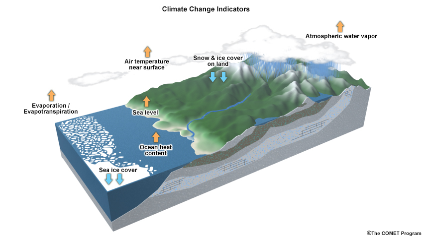
What are we certain about? On a global scale we know that sea and land ice volume is decreasing as average temperature, evaporation, and atmospheric water vapor are increasing.

What are we pretty sure about? There are likely to be some regional differences from the global averages, but most regions are likely to experience the following:

• more frequent wet and/or dry extremes brought about by warmer temperatures,

• increased evapotranspiration, and

• changes to precipitation intensity, distribution, and phase (liquid versus frozen).

These changes may lie outside the range of observations in the period of record, and will need to be taken into account in water research and resources planning.

Trends Impacting Water and Environmental Resources Planning

The following observed and/or projected trends have an impact on planning for water and environmental resources.

• Global average temperature has been warming and will continue to warm through the 21st century

• Short-term natural cycles of increased warming interspersed with cooling (or slower warming) will be superimposed on overall long-term warming

• Average snow cover and snowpack in the United States is likely to decrease through the 21st century

• Precipitation extremes (wet and dry) are likely to continue increasing through the 21st century, with some regional trends toward either more wet or more dry

These climate trends have, and will continue to have, impacts on water resources.

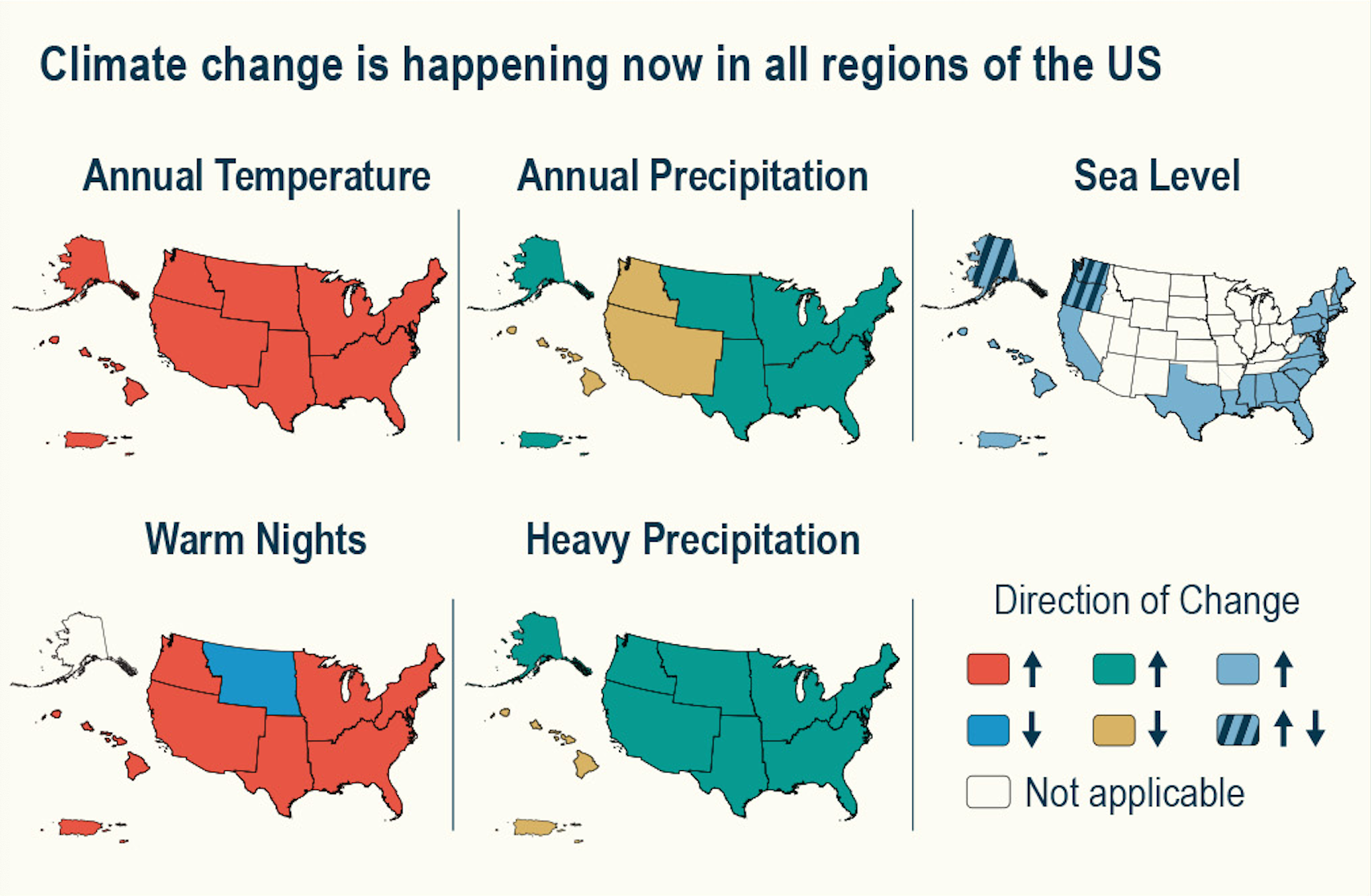
The need for understanding the influence of climate change on the U.S. water sector, its impacts, and imperative for informed decision-making across the U.S. is highlighted in The Fifth National Climate Assessment (NCA5; https://nca2023.globalchange.gov/; see Chapter 2 for more in-depth discussion) produced by the U.S. Global Change Research Program, with the following key message, “The effects of human-caused climate change are already far-reaching and worsening across every region of the United States.” In addition, the NCA5 states that, “Changes in multiple aspects of climate are apparent in every U.S. region … warming is apparent in every region … average annual precipitation is increasing in most regions, except in the Northwest, Southwest, and Hawai’i, where precipitation has decreased … heavy precipitation events are increasing everywhere except Hawai’i and the U.S. Caribbean” (see NCA5 for further information on how CC affects the U.S.’s physical Earth systems, current and future risks, and what can be done to reduce those risks, in each of the 10 NCA5-defined regions.

From NCA5

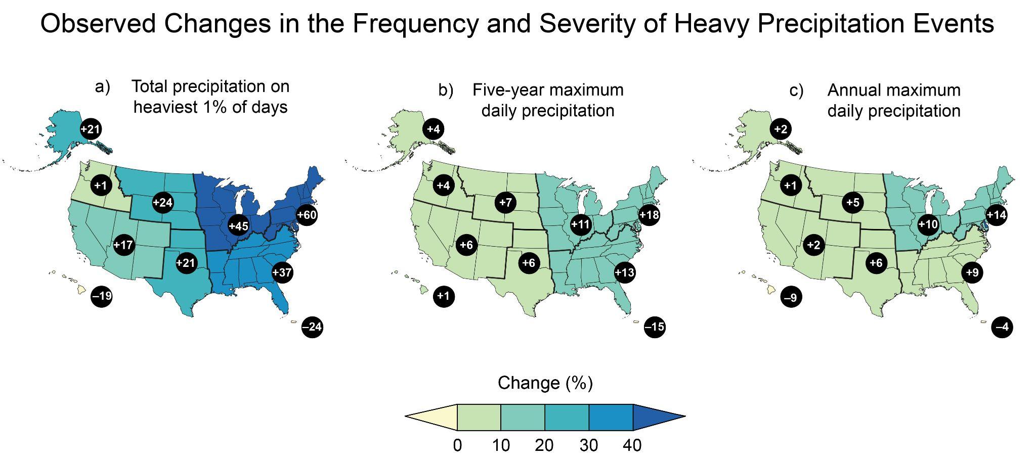
The frequency and intensity of heavy precipitation events have increased across much of the United States, particularly the eastern part of the continental U.S., with implications for flood risk and infrastructure planning. Maps show observed changes in three measures of extreme precipitation: (a) total precipitation falling on the heaviest 1% of days, (b) daily maximum precipitation in a 5-year period, and (c) the annual heaviest daily precipitation amount over 1958–2021. Numbers in black circles depict percent changes at the regional level. Data were not available for the U.S.-Affiliated Pacific Islands and the U.S. Virgin Islands. Figure credits: from NCA5, (a) adapted from Easterling et al. 2017; (b, c) NOAA NCEI and CISESS NC.

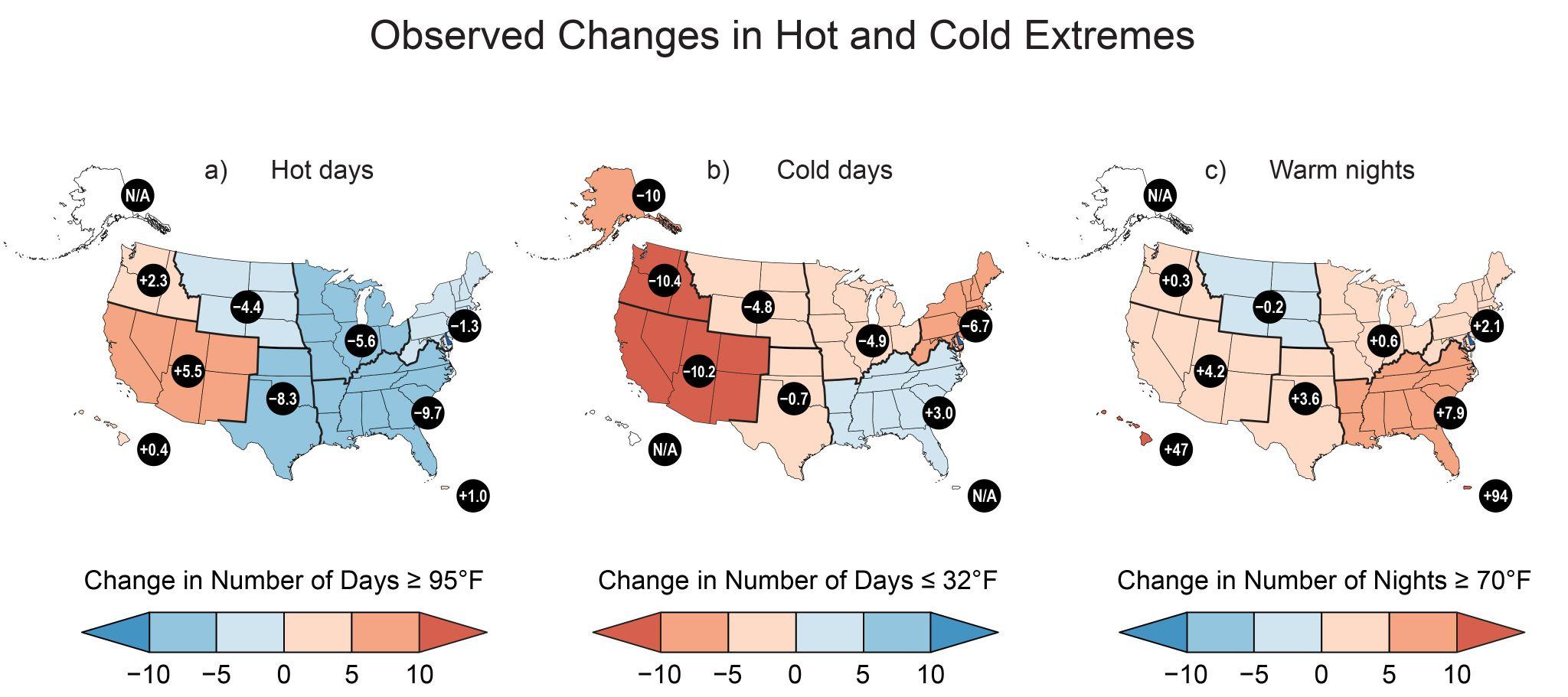
Over much of the country, the risk of warm nights has increased while the risk of cold days has decreased. The risk of hot days has also increased across the western U.S. This figure shows the observed change in the number of (a) hot days (days at or above 95°F), (b) cold days (days at or below 32°F), and (c) warm nights (nights at or above 70°F) over the period 2002–2021 relative to 1901–1960 (1951–1980 for Alaska and Hawai’i and 1956–1980 for Puerto Rico). Data were not available for the U.S.-Affiliated Pacific Islands and the U.S. Virgin Islands. Figure credit: from NCA5, Project Drawdown, Washington State University Vancouver, NOAA NCEI, and CISESS NC.

Precipitation Variability and Trends – Unlike temperature, it is much more difficult to detect a steady global trend in precipitation, although trends toward wetter or drier conditions exist in certain regions. A warmer atmosphere can hold more water vapor. This can lead to longer precipitation-free periods, but also more intense precipitation when it does rain or snow.

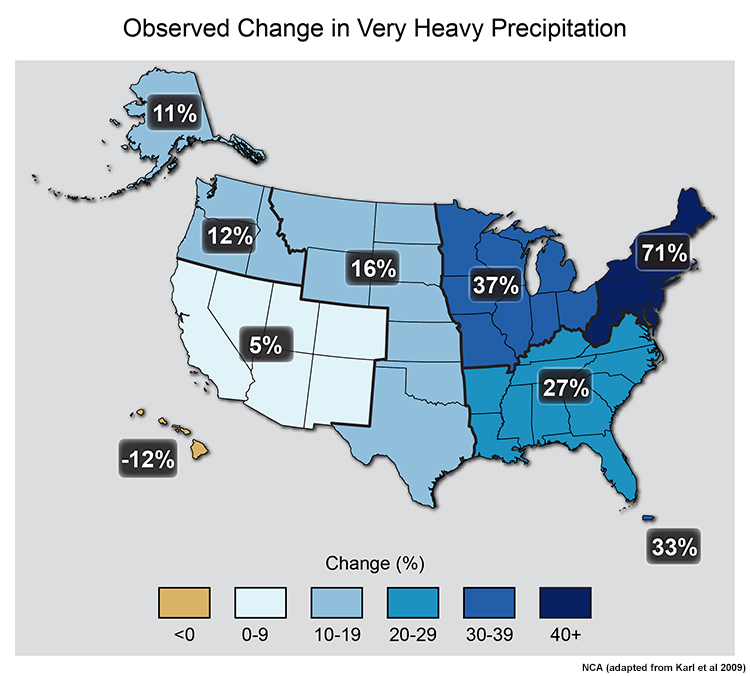
Percent increases in the amount of precipitation falling in the heaviest 1% of all daily events (1958 to 2012) for different regions of the contiguous United States. The changes in the Southwest are likely masked by high natural variability. (Figure source: from NCA5, updated from Karl et al. 2009).

Observations in the United States from 1958-2012 show that the amount of precipitation falling in the heaviest 1% of daily events is increasing in all states except Hawai’i. The Northeast and upper Midwest exhibit the most notable increase in intense precipitation. The interrelationships between precipitation and other climate variables are important to hydrology. Temperature affects the hydrological cycle due to its influence on evapotranspiration, water temperature, precipitation phase, and melting, among other things.

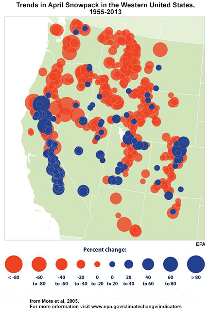
In the western part of the contiguous United States, the observed trend in April 1st snowpack is decreasing in a majority of locations, especially the northern Rocky Mountains and Pacific Northwest.

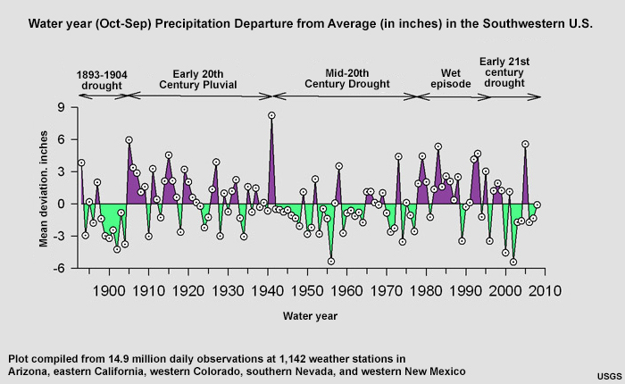
water year precipitation of the Southwest U.S.A., 1894-2008. Multidecadal wet and dry episodes are labeled. Precipitation is expressed as mean deviation from individual station averages. USGS

Historic observations in the southwestern United States show multi-year periods of both positive and negative annual precipitation anomalies rather than a long-term trend in precipitation amount. Because the warmer temperatures of recent decades can contribute to greater evapotranspiration, the negative precipitation anomalies may result in more severe dr ought compared to similar negative precipitation anomalies of the early 20th century.

Trends in Extremes – Observation-based studies show that natural variability in temperature continues on the background of overall warming. Precipitation trends show a tendency for more extremes, both wet and dry, on a global scale, with some regional trends toward either wetter or drier overall.

Typically, water research, resources planning, operations, and management already consider natural climate variability. As we move into the future, natural climate variability will continue, but it will be superimposed on a trend caused by climate change. As the “background” climate warms the global mean, the extremes associated with natural variability may reach magnitudes rarely or never before seen in the observed record.

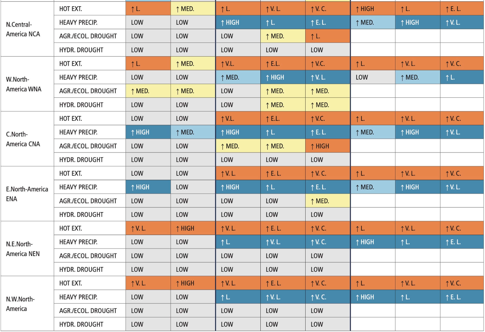
Regional Information on Extremes – The table below was taken from IPCC AR6 (Seneviratne et al. 2021) and provides summary regional assessments for hot extremes (HOT EXT.), heavy precipitation (HEAVY PRECIP.), agriculture and ecological droughts (AGR./ECOL. DROUGHT), and hydrological droughts (HYDR. DROUGHT). It shows the direction of change and level of confidence in the observed trends (column OBS.), human contribution to observed trends (ATTR.), and projected changes at 1.5°C, 2°C and 4°C of global warming for each AR6 region. Projections are shown for two different baseline periods: 1850–1900 (pre-industrial) and 1995–2014 (modern or recent past) (see Seneviratne et al., 2021 Section 1.4.1 for more details). Direction of change is represented by an upward arrow (increase) and a downward arrow (decrease). Level of confidence is reported for LOW: low, MED.: medium, HIGH: high; levels of likelihood (only in cases of high confidence) include: L: likely, VL: very likely, EL: extremely likely, VC: virtually certain. Dark-orange shading highlights high confidence (also including likely, very likely, extremely likely, and virtually certain changes) increases in hot-temperature extremes, agricultural and ecological drought, or hydrological droughts. Yellow indicates medium confidence increases in these extremes, and blue shadings indicate decreases in these extremes. High confidence increases in heavy precipitation are highlighted in dark blue, while medium confidence increases are highlighted in light blue. No assessment for changes in drought with respect to the 1995–2014 baseline is provided, which is why the respective cells are empty.