Advanced Plotting#
BEFORE BEGINNING THIS EXERCISE - Check that your kernel (upper right corner, above) is NPL 2026a. This should be the default kernel, but if it is not, click on that button and select NPL 2026a.
This activity was developed primarily by Mauricio Rocha and Gustavo Marques.
Setting up the notebook#
Here we load modules needed for our analysis
# loading modules

# %load_ext watermark # this is so that in the end we can check which module versions we used
%load_ext autoreload

import warnings
warnings.filterwarnings("ignore")

import datetime
import glob
import os
import warnings
import dask
import dask_jobqueue
import distributed
import matplotlib as mpl
import matplotlib.pyplot as plt
import numpy as np
import xarray as xr
from matplotlib import ticker, cm
from cartopy import crs as ccrs, feature as cfeature
import cartopy
Get the data#
# Set your casename here:
casename = 'g.e30_a09a.GJRAv4.TL319_t233_wgx3_hycom1_N75.2026.020'

# Here we point to the archive directory:
pth = f'/glade/derecho/scratch/gmarques/archive/{casename}/ocn/hist/'

# Load data:
flist = glob.glob(pth + casename + '.mom6.h.native.000?-??.nc')
ds = xr.open_mfdataset(flist, compat='override', coords='minimal')
ds
Exercise 1#
Maximum mixed-layer depth for the winter months in the northern hemisphere (January, February, and March) and in the southern hemisphere (July, August, and September)
# July, August, and Septemper (JAS)
JAS = ds.mlotst_max.where(ds.time.dt.month.isin([7, 8, 9]), drop=True).mean(dim="time")

# January, February, and March (JFM)
JFM = ds.mlotst_max.where(ds.time.dt.month.isin([1, 2, 3]), drop=True).mean(dim="time")
# Create a new array
winter=JFM.copy()

# Since the variable winter already contains the data for the Northern Hemisphere, we will now add the data for the Southern Hemisphere
winter.loc[-90:0,:]=JAS.loc[-90:0,:]
plt.figure(figsize=(8,6));
ax = plt.axes(projection=ccrs.Robinson());
orig_map=plt.cm.get_cmap('turbo')
scale_color=orig_map.reversed()
cf=(winter).plot.pcolormesh(ax=ax,
                              vmax=800,vmin=0,
                              transform=ccrs.PlateCarree(),
                              x='xh',
                              y='yh',
                              cmap=scale_color,
                              add_colorbar=False,
                           )
ax.coastlines()
ax.add_feature(cartopy.feature.LAND)
ax.gridlines(crs=ccrs.PlateCarree(), draw_labels=True,
                  linewidth=2, color='gray', alpha=0.5, linestyle='-')
cbar = plt.colorbar(cf, ax=ax, shrink=0.5, pad=0.1, ticks=np.arange(0,800,100), label='mlotst_max [m]')
plt.title('Maximum Mixed-Layer Depth for the Winter', fontsize=14)
#plt.savefig('advanced_plot_1.png', bbox_inches='tight')# uncomment this to save your figure
Click here for the solution
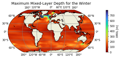
Figure: Plotting solution.
Exercise 2#
Calculate the time average of heat content (HC) per unit area from the temperature for the upper 2000m. Equation: $\(\rm{HC = \rho_\theta~C_p~\int_{z_2}^{z_1}T(z)~dz},\)$ where:
\(\rm{HC}\) is heat content (\(\rm{J~m^{-2}}\)),
\(\rho_\theta\) is the sea water density (\(\rm{kg~m^{-3}}\)),
\(\rm{C_p}\) is the sea water specific heat (\(\rm{J~kg^{-1}~^{\circ}C^{-1}}\)),
\(\rm{dz}\) is the cell thickness (\(\rm{m}\)),
and \(T\) is the temperature (\(\rm{^{\circ}C}\)).
For this exercise we want data on the z-grid (*.mom6.h.z.000?-??.nc) instead of the native grid (*.mom6.h.native.000?-??.nc).
%%time
# how quick this is depends among other things on the availability of workers on casper
# you can check progress by clicking on the link for the cluster above which will show you the dask dashboard
full_pth = pth + casename + '.mom6.h.z.000?-??.nc'  #also might want to use just some years not all
ds = xr.open_mfdataset(full_pth, parallel=True)
ds #print some meta-data to screen
ds_HC=ds['thetao'].sel(z_l=slice(0,2000))*ds['h'].sel(z_l=slice(0,2000)) # Select the depth and multiply by dz. Unit: oC.m
ds_HC=ds_HC.sum('z_l')                                                   # Sum in depth
ds_HC=ds_HC*1026                                                         # Multiply it by the sea water density. Unit: oC.kg.m-2
ds_HC=ds_HC*3996                                                         # Multiply it by the sea water heat specific. Unit: J.m-2
ds_HC=ds_HC.mean('time')                                                 # Take the time average
plt.figure(figsize=(8,6))
ax = plt.axes(projection=ccrs.Robinson())
orig_map=plt.cm.get_cmap('turbo_r')
scale_color=orig_map.reversed()
cf=(1e-9*ds_HC).plot.pcolormesh(ax=ax,
                              transform=ccrs.PlateCarree(),
                              vmin=0,
                              vmax=80,
                              x='xh',
                              y='yh',
                              cmap=scale_color,
                              add_colorbar=False,
                           )
ax.coastlines()
ax.add_feature(cartopy.feature.LAND)
ax.gridlines(crs=ccrs.PlateCarree(), draw_labels=True,
                  linewidth=2, color='gray', alpha=0.5, linestyle='-')
cbar = plt.colorbar(cf, ax=ax, shrink=0.5, pad=0.1, label='HC [$10^9$ J m$^{-2}$]')
plt.title('Heat content per unit area for the upper 2000 m', fontsize=14)
#plt.savefig('advanced_plot_2.png', bbox_inches='tight')# uncomment this to save your figure
Click here for the solution
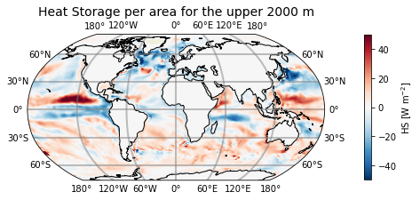
Figure: Plotting solution.