Diagnostics#
These activities have been tested and updated by members of the CESM Tutorial Committee.
Once the CESM model has been run and the output data has been transfered to the short term archive directory the real job of understanding how the simulation ran and what it means from a scientific perspective begins.
By this point you have run a number of simulations and have looked at model output using ncview. In this lab you will go beyond ncview by using Python plotting and analysis methods in Jupyterhub to produce additional diagnostic results. There is also a complete CESM diagnostics system under active development called CUPiD that you will get to try out, and which will be released with CESM3.
Finally, please note that there are many other CESM analysis tools and projects available as well, but not all will be covered here.
To start running the Jupyter Notebooks provided for this tutorial, follow the steps below.
Step 1. Download CESM Tutorial notebooks with Git Clone#
First we will change into the home directory and then we will use the git clone command to download the CESM Tutorial diagnostics notebooks.
cd
Download the cesm code to your code workspace directory as CESM-Tutorial:
git clone https://github.com/NCAR/CESM-Tutorial.git CESM-Tutorial
Step 2. Login to Jupyter#
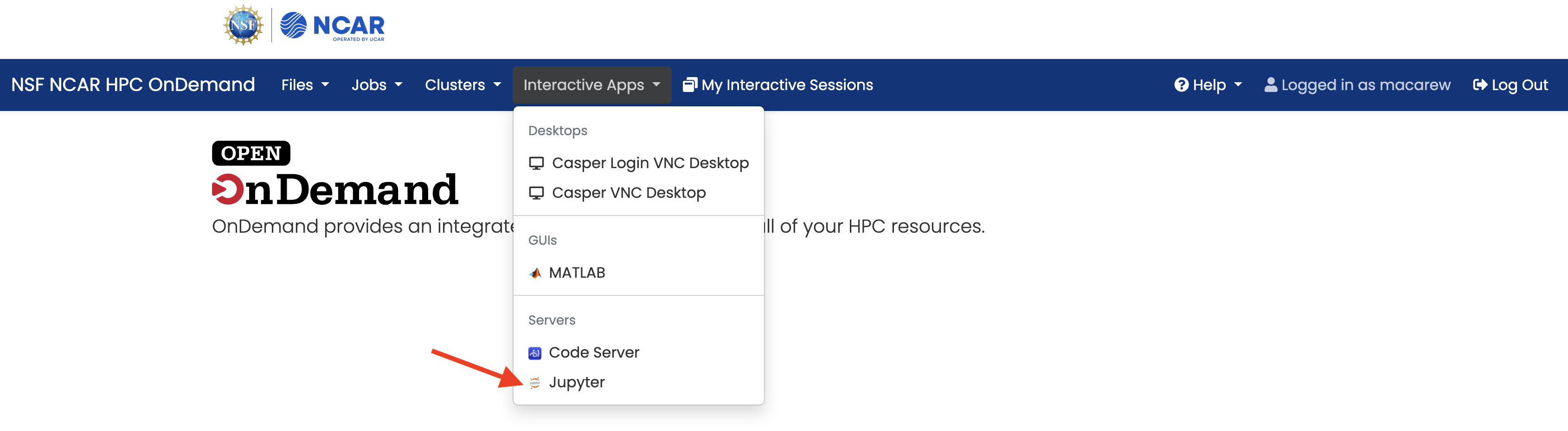
To access JupyterLab, first go to the NCAR OnDemand website, which may require logging in with your CIT username and password (i.e. the one you use for Derecho). Once you are on the landing page, click on the “Interactive Apps” drop-down menu at the top, and then select “Jupter”
This will take you to a page where you’ll need to enter information related to your Jupyter job. For this lab, you’ll need to manually set the following:
Jupyter job Settings |
|
|---|---|
Resource Selection |
Casper PBS Batch |
Queue or Reservation |
casper |
Project Account |
UESM0016 |
Wall Time in Hours |
3 |
which should be located here:
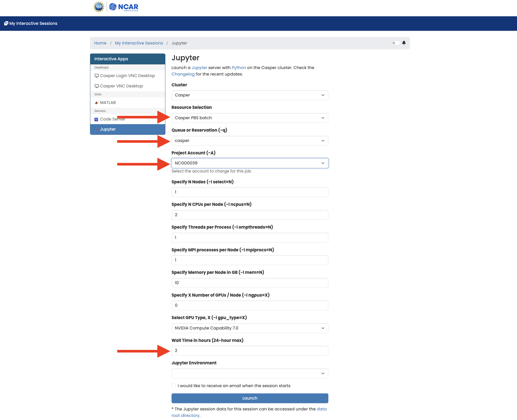
Once you are done changing the settings, click on the Launch button, which should take you to another screen stating that your job is in the queue, and/or “Starting”. After a couple minutes there should eventually be a Connect to Jupyter button, as shown below.
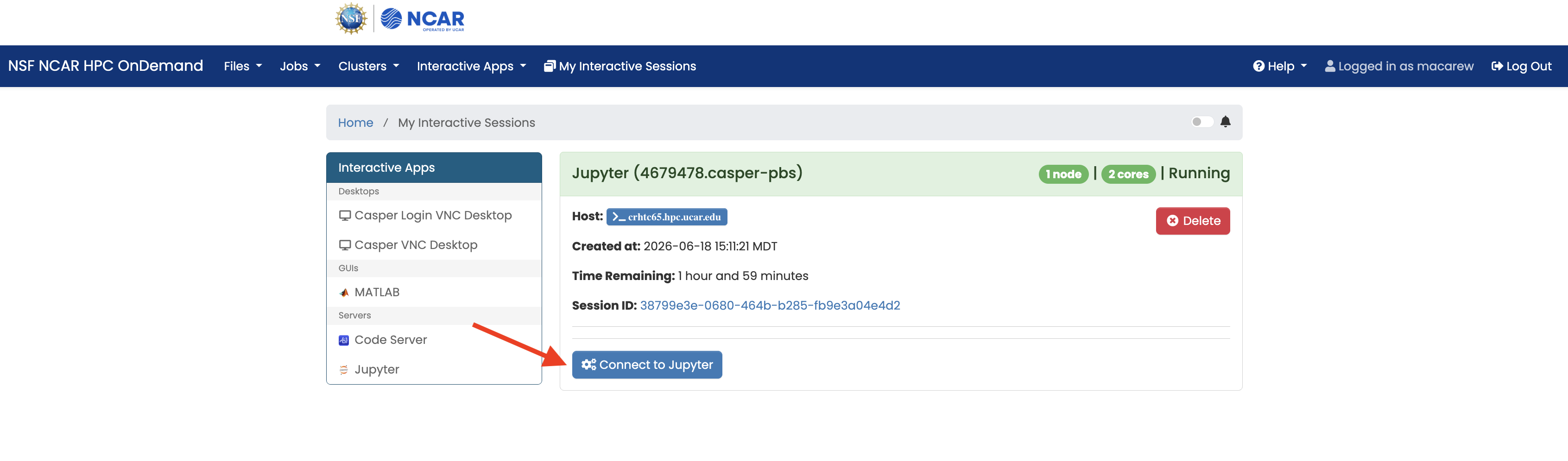
Click on that button, and you should now have access to a running JupyterLab session!
Step 3. Open a Diagnostics Notebook#
When your JupyterLab session opens you should be in your home directory on the NCAR HPC. In Step 1 you cloned the “CESM-Tutorial” repository, which has the notebooks you will run in this activity.
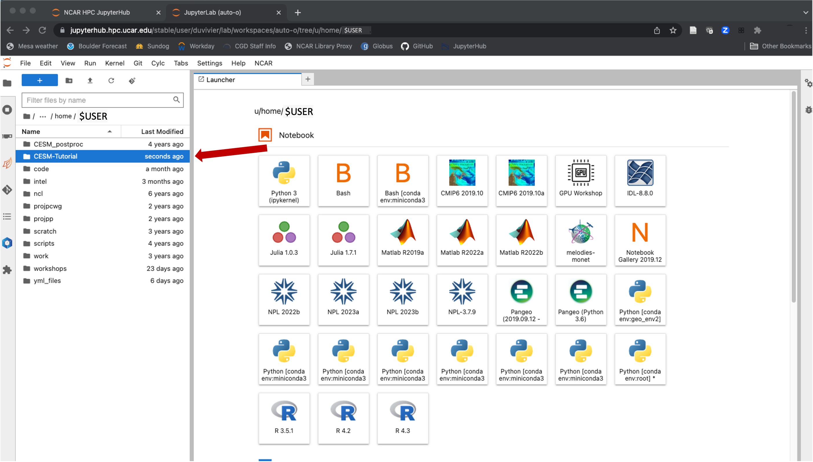
To get to the Diagnostics notebooks, double click the following sequence of folders:
CESM-Tutorial
notebooks
diagnostics
Click on the folder for the model component that you are interested in running (e.g. cam), or the
cupid.ipynbfile if you are interested in trying CUPiD.Click on the
basics.ipynbnotebook (see arrow on left, below)
The final path in your browser url line for the following example should be:
$USER/CESM-Tutorial/notebooks/diagnostics/cam/basics.ipynb
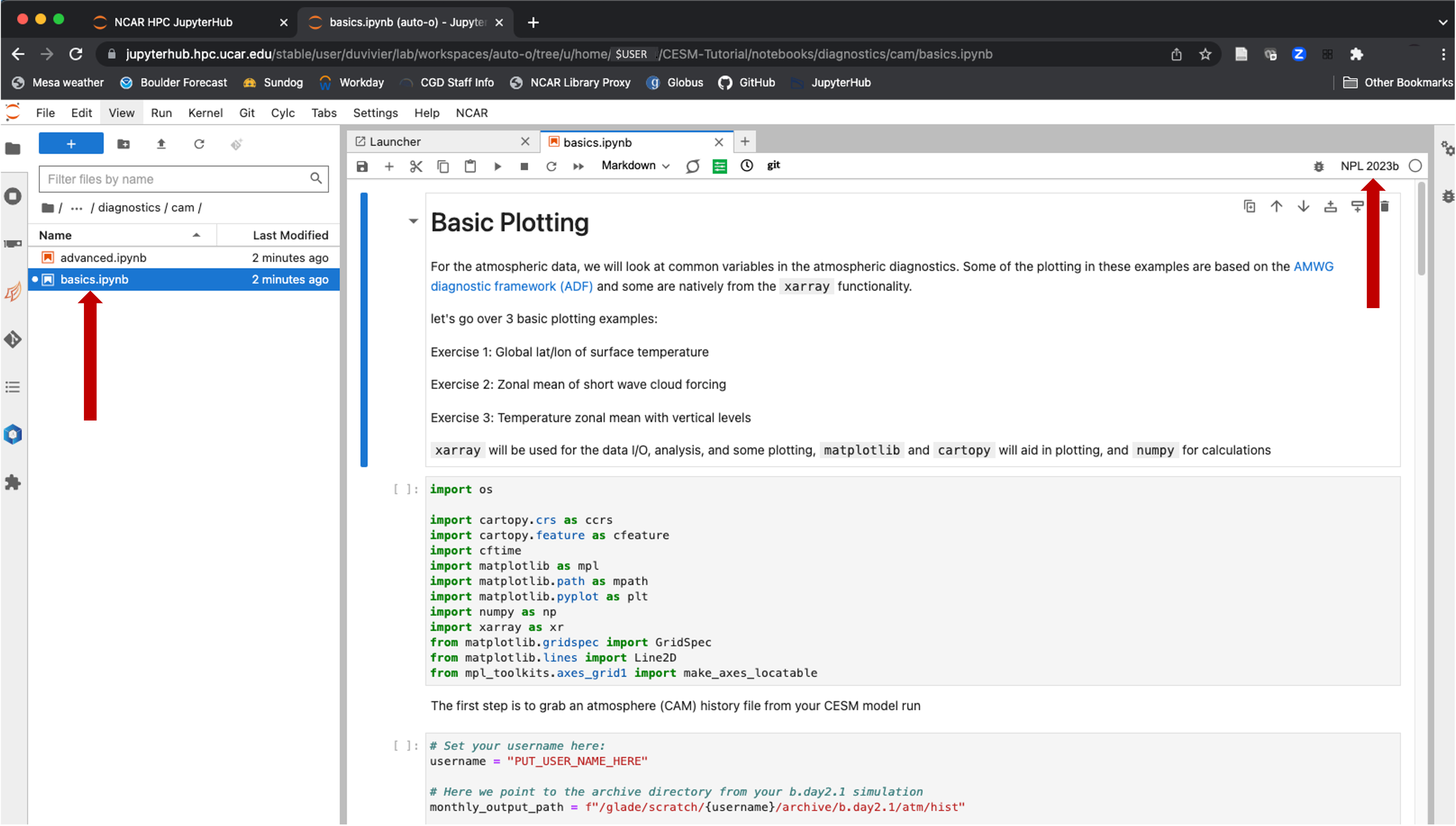
Step 4. Check Your Notebook Kernel#
Check your kernel (see arrow in upper right corner, above). It should be either NPL 2025a or NPL 2025b. You should use the specified kernel for any diagnostics you do during the tutorial as it is a default environment available on NCAR HPC and the notebooks here have been tested so that they work with that particular kernel for the analysis environment. We have set the default kernels and specifiy what they should be in each component notebook. However, if you need to change it click on the kernel button and select the correct kernel.
Step 5. Run Jupyter Notebook Cells#
To run a Jupyter cell
Type your command into the cell
To execute the command:
Press shift+return
OR- Select the cell then click the 'play' button at the top of the window (see red arrow, above)All figures will be rendered in the Jupyter Notebook, so there is no need to open any other window for this portion of the lab activities.