Ocean

The ocean component of CESM is the Parallel Ocean Program (POP).

It can be useful for people interested in ocean science to run simulations with only active sea ice and ocean components and atmospheric forcing. In this exercise, you will learn how to run one of these ice-ocean simulations.

This exercise was created by Gustavo Marques.

Learning Goals

• Student will learn what a G compset is, the types of forcing available to run one, and how to run one.

• Student will learn how to make a namelist modification that turns off the overflow parameterization and compare results with a control experiment.

• Student will learn how to make a source code modification that changes zonal wind stress and compare results with a control experiment.

• Student will learn what a G1850ECO compset is and compare it to the G compset.

Exercise Details

• This exercise uses the same code base as the rest of the tutorial.

• You will be using the G compset at the T62_g37 resolution.

• You will run a control simulation and three experimental simulations. Each simulation will be run for one year.

• You will then use ‘ncview’ (http://meteora.ucsd.edu/~pierce/ncview_home_page.html) to evaluate how the experiments differ from the control simulation.

Useful POP references

CESM POP User’s Guide

CESM POP Discussion Forum

What is a G case?

The G compset has active and coupled ocean and sea-ice components. The G compset requires boundary forcing from the atmosphere. The G compset is forced with atmospheric data that does not change interactively as the ocean and sea-ice evolve in time. The land and land ice are not active during a G compset experiment and the runoff is specified.

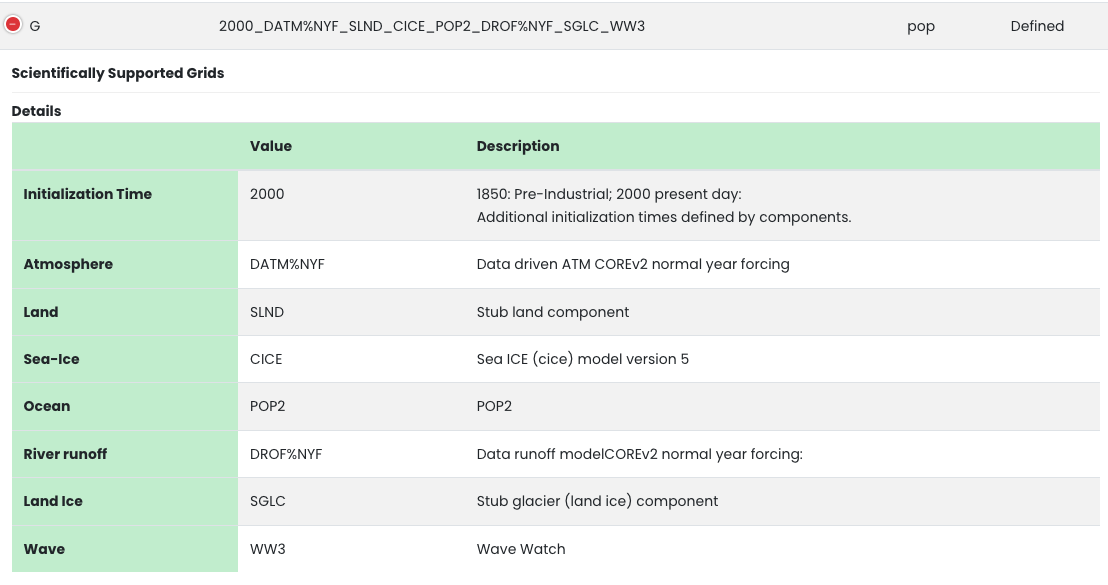
Figure: G compset definition.

Component Set Definitions

G Compset forcing data

There are two types of temporal forcing for G compsets:

• Normal Year Forcing (NYF) is 12 months of atmospheric data (like a climatology) that repeats every year. NYF is the default forcing.

• Interannual varying forcing (GIAF) is forcing that varies by year over the time period (1948-2017).

There are two datasets that can be used for G compsets:

• JRA55-do atmospheric data (Tsujino et al. 2018)

• Coordinated Ocean-ice Reference Experiments (CORE) version 2 atmospheric data (Large and Yeager 2009).

In these exercises we will use the CORE NYF.

Post processing and viewing your output

1. You can create an annual average of the first year’s data for each simulationg using the ncra (netCDF averager) command from the netCDF operators package (NCO).

ncra $OUTPUT_DIR/*.pop.h.0001*nc $CASENAME.pop.h.0001.nc

2. Create a file that contains differences between each of the experiments and the control simulation

ncdiff $CASENAME.pop.h.0001.nc $CONTROLCASE.pop.h.0001.nc $CASENAME_diff.nc

3. Examine variables within each annual mean and the difference files using ncview

ncview $CASENAME_diff.nc

4. You can also look at other monthly-mean outputs or component log files.